Chapter Introduction: Modeling
The essence of machine learning (ML) involves fitting a mathematical function to define the relationship between a target variable and a set of predictor features. In applied data science, the end purpose of such a function is to predict the outcome of new, never-before-seen cases. The applications of ML are wide-ranging and well-documented. The goal of this chapter is not to explain the inner workings of ML algorithms. Myriad resources exist to accomplish that task. Rather, this chapter will show how to effectively implement and tune popular ML algorithms.
Regression vs. Classification
The two most popular types of ML algorithms are classification and regression. Regression algorithms predict a continuous outcome, such as the price of a stock or the closing price of a house. A classification model predicts a discrete label, such as whether someone will opt out of an email campaign or whether someone will buy a product. When building a classification model, we oftentimes prefer to predict the probability of an observation being in a given class. For example, we might predict the probability of a person opting out of an email campaign. More on predicting strong probabilities in chapter 11.
Our customer churn model is a classification task. We will develop a model to predict the probability of a person canceling their monthly subscription. This model will be the core of what we do. Without it, we have nothing that is actionable!
Training and Testing Sets
When building a machine learning model, we want to train it on a certain set of data (training set) and validate it on a distinct, separate set of data (testing data). Completely holding out a portion of data is vital. Checking the predictive power on our test set gives us an idea of how our model will generalize to brand new observations in production. Analyzing the predictive performance on our test set is vital to assessing the strengths and weaknesses of our models and for selecting the final model(s) we want to put into production. We will discuss this topic more in chapter 12.
For our problem, we can randomly assign observations to our test set. Generally, we assign somewhere between 10-30% of our observations to the test set. Setting the percentage is a mix of art and science. Oftentimes, we'll rely on a rule of thumb that we have employed for similar projects in the past (e.g. 25% goes to the test set). The size of our test set should be influenced by the size of our overall dataset. We need a test set that is large enough to be reliable. If we only have, say, 10 observation in our test set, most of our evaluation statistics won't be reliable (to note, the situation is a bit different for time-series problems). If we have a huge dataset, we can be fine assigning a smaller percentage of observations to our test set (e.g. 10%). However, if our dataset is smaller, we likely we need a larger percentage. That said, we still need ample training data. A balance exists - and finding it can oftentimes be an art. However, we can use learning curves to help inform our decision, which we will cover in an upcoming section.
To create a train-test split, we can use the following function, which will be placed in helpers/model_helpers.py
Defining Cross Validation
Cross validation is a core concept in machine learning. Simply, cross validation splits our training data into new training and testing sets in a rotating fashion. To begin this process, we select the number of folds (referred to as k) we want in our cross validation scheme. To keep it simple, we'll select a small number of 3 folds in this example. Selecting k=3, we randomly split our data into three folds. We then fit three separate models, with each fold being used as the testing set one time.
- Fit 1: folds 1 and 2 are used for training, and fold 3 is used for testing.
- Fit 2: folds 2 and 3 are used for training, and fold 1 is used for testing.
- Fit 3: folds 1 and 3 are used for training, and fold 2 is used for testing.
Why would we want to use cross validation? The main reason is that it can give us a better idea of how our model will generalize to new data. Rather than scoring our model on only one holdout set of data, we do so on multiple sets. It's possible that our model may score well on a certain holdout set simply by chance. Lucky splits happen. By performing the holdout evaluation multiple times and taking the average, we get a better view of the actual error we might expect "in the wild". Cross validation is crucial. It gives us a fuller picture and more confidence that model evaluation results are not function of a lucky or unlucky random split.
We primarily use cross validation when determining the parameters for our model. As a simple example, let's say we want to see if a max_depth of 10 or 15 performs better for our Random Forest algorithm. If we used k=3, we would build three models, as described above, with the max_depth set to 10 and take the average score on the testing sets (remember, each fold is used for testing one time). We would then build three models with the max_depth set to 15 and take the average score on the testing sets. The max_depth setting with the best average score on the testing sets would be declared the winner. Again, by engineering multiple test sets, we have more confidence in the evaluation scores we get.
The above process is elegant. It preserves the integrity of our full testing set, which we discussed in the last section. The testing set should never be used to try hyperparameter combinations. Rather, we should always leverage cross validation to repurpose our training set to tune hyperparameters. Cross validation helps us make better use of our data.
What's a good number for k? Well, it depends. A value is 3 is the floor - don't go any lower than that. You might see values as high as 12 or 13 but rarely anything higher. The size of your training set plays a huge role. If you have a small training set and you set k to a high value, your testing sets will be small and the results less reliable. Likewise, setting k to a high value will increase the time it takes to tune your models. If you have a huge dataset, you'd probably be good setting k to something like 5, knowing you'll have good-sized test sets. No "right" answer exists. Through experience, you'll find what works well for your modeling tasks.
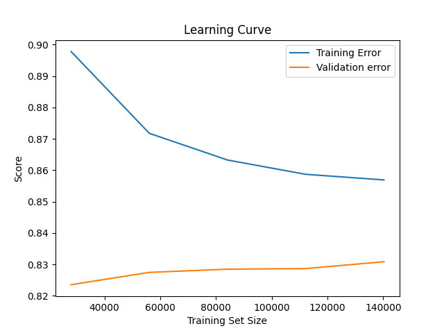
Plotting Learning Curves
A learning curve shows us the diminishing returns of adding more training data. Logically, our algorithm will cease improving at some point as we add more data. This approximate point will be highly contingent on the problem at hand. We can use such a point to help inform roughly how large our training set should be. Fortunately, we can leverage scikit-learn to plot our learning curve. Let's create utilities/learning_curves.py and add the following code to it. Recall the utilities directory houses ancillary, one-off processes.
We see that our training error goes down and then stabilizes. The higher scores on less data are likely due to statistical noise. With small samples sizes, we should have less confidence in our scores. However, we care more about the validation error. We see that it generally goes up as we increase the training data size. (We're using ROC AUC as our scoring metric, and we want this metric to be as high as possible). This finding means we should have as large of a training set as we can - but we still need to balance having a large enough testing set to be stable. To note, for our learning curve, we used an un-tuned model and bare-bones preprocessing. We'll get better performance with improved tuning and cleaning. Also, we are clearly overfitting the training set as our training error and validation error differ quite noticeably.
Our Scikit-Learn Modeling Pipeline
In previous chapters, we have mentioned our modeling pipeline multiple times. This is where much of the magic happens: our preprocessing and modeling steps get defined and ordered. Please review the pipeline below. We will then discuss each step in turn.
At a high level, we have four main components to our pipeline.
- A pipeline of preprocessing steps for our numeric features.
- A pipeline of preprocessing steps for our categorical features.
- A ColumnTransformer object that combines the previous two pipelines.
- A final pipeline that combines the ColumnTransformer with preprocessing steps that will be applied to all columns along with a machine learning model.
Let's first review our numeric_transformer.
- Our first few steps are mouse_movement_clipper, propensity_score_clipper, completeness_score_clipper, and profile_score_clipper, and average_stars_cliper. These steps clip suspect feature values we discovered during exploration. To note, sklearn's FunctionTransformer allows us to apply a plain Python function in a pipeline.
- Our next step is ratio_creator, which creates a ratio of two columns, profile_score and activity_score.
- The log_creator step takes the logarithm of our columns. This is actually tunable step (see parameter grid).
- The dict_creator steps converts the data to a dictionary, which is necessary for the DictVectorizer.
- The dict_vectorizer creates a feature-value mapping. Creating a mapping in such a fashion keeps our model from breaking if a new column gets added without our knowledge. The DictVectorizer also has an attribute that captures our column names before they disappear. In the next step, our data becomes a numpy array, which has no column names.
- The imputer steps fills in missing values with the column mean. We could tune this parameter if we wanted.
- The scaler scales the data so that each column has the same scale.
- The feature selector keeps a certain percentage of features based on the results of an ANOVA test. We tune this parameter.
Let's now review our categorical_transformer.
- The first step, date_transformer, casts acquired_date to be of type pandas datetime.
- The next step, month_extractor, extracts the month from acquired_date.
- The quarter_extractor step takes the month and converts into a quarter of the year.
- The year_extractor step extracts a year from acquired_date.
- The date_dropper step drops our date column, as we don't want to one-hot encode it in a few steps.
- The imputer steps fills in null categorical values with a specified string. We are using our own function and not scikit-learn's imputer. In this case, we are only filling in categorical nulls with a static value, so we don't risk feature leakage. Likewise, we don't want to lose our column names at this stage by converting our data into an array.
- The category_combiner step combines sparse category levels. This is another preprocessing step that we tune.
- The dict_creator steps converts the data to a dictionary, which is necessary for the DictVectorizer.
- The dict_vectorizer is how we one-hot encode our features. Doing our one-hot encoding in this fashion has a big advantage over something like pandas get_dummies(). If a category level is added, our model won't break. The DictVectorizer seamlessly handles new categories, which is a huge plus in a production setting. Likewise, the DictVectorizer also has an attribute that captures our column names before they disappear.
- The feature selector keeps a certain percentage of features based on the results of an chi-squared test. We tune this parameter. We have two feature selector mechanisms because we want to run different statistical tests based on type of data (numeric vs. categorical).
Whew! That's a lot. Our next object is the preprocessor. This part is simple: we apply the numeric_transformer to our numeric columns, and we apply our categorical_transformer to our categorical columns.
Lastly, we create our main pipeline.
- The first step is the data_mapper, which relies on a dictionary of feature-datatype mappings in our config file. The dictionary mapping represents our expected universe of features and their associated datatypes. One of the downsides of using the ColumnTransformer is that it expects the same columns in production as it does during training. If a column is added or subtracted, our pipeline will break. This is not desireable. The data_mapper essentially alleviates of this concern. If an unexpected column is added, it will get dropped. If an expected column is missing, it will be added with all null values. Likewise, it will ensure all features have the expected datatypes. This doesn't so much help us during training, but it is nice functionality to have when we go to production. In production, we want our pipeline to handle everything, including all preprocessing. We simply want to throw our data into our pipeline and get a prediction back.
- The second step in the main pipeline is the preprocessor described above, which is applied to the numeric and categorical features, respectively.
- The variance_thresholder removes features that only have a single value.
- Lastly, our machine learning model is applied.
One item you might notice is that we are applying FeaturesToDict and DictVectorizer twice. Why is this? In the numeric_transformer, the imputer step turns our dataframe into a numpy array, and we lose our column names. The DictVectorizer has a feature_names_ attribute, which is the way we can take a snapshot of our feature names before we lose them in the pipeline. Likewise, in the categorical_transformer, we use the DictVectorizer to one-hot encode our features. The DictVectorizer will tell us the names of all of our dummied features.
Pipeline Variant: Handling Imbalanced Data
Our target (churn or not churn) is imbalanced. Far fewer people churn than do not churn. In general, in some select cases, we might benefit from artificially balancing our classes. We can only know through experimentation. Some important cautions exist when we want to re-balance our target class. First, we are forced to either remove data or artificially create data. There are smart ways we can accomplish either task, but that doesn't mean those are risk-free actions. Second, since we often care about predicting calibrated probabilities, messing with our class balance can hinder our calibration. Caveat emptor.
As alluded, we can either remove observations (undersampling) or create synthetic observations (oversampling). Though altering our class balance can be risky for the reasons described, there could be cases where we must undersample. This might occur when we have tons of data but only limited computational resources and the class balance is severe. That said, we need to be careful where we perform the undersampling or oversampling. We must only perform this type of operation on the training fold during cross validation. If we undersample or oversample any data that is used for testing or validation, we are not going to get an accurate view of how our model will generalize in a production setting. You don't undersample or oversample in production! In the same vein, you don't undersample or oversample test data.
Unfortunately, we cannot perform undersamping or oversampling in a scikit-learn pipeline. However, we can do so in an imbalanced-learn pipeline. To implement undersampling of the negative (majority) class, we can make the following changes.
In modeling/pipeline.py, remove the following import: from sklearn.pipeline import Pipeline. In its stead, include the following import statements.
        from imblearn.pipeline import Pipeline

        from imblearn.under_sampling import RandomUnderSampler
Further, we'll need to add the following tuple as the first item in our pipeline.
('undersampling', RandomUnderSampler(sampling_strategy=create_undersampling_dict))
create_undersampling_dict is our undersampling strategy, which we must be passed as a callable and must return a dictionary. The function is defined in helpers/model_helpers, so we'll also need to import it in modeling/pipeline.py. It simply randomly eliminates 50% of the negative observations.
from collections import Counter


    def create_undersampling_dict(y):

   """

   Creates a dictionary for undersampling the negative class


   param y: the y target series

   :returns: dictionary

   """

   counter = Counter(y)

   neg_count = counter.get(0)

   neg_adjusted_count = int(neg_count * 0.5)

   pos_count = counter.get(1)

   return {0: neg_adjusted_count, 1: pos_count}
After implementing these changes, if we run modeling/train.py, we will be training our models using undersampling. Again, this can be a risky choice as it can mess with proper calibration, so we need to be careful and closely inspect the effects on our model.
Pipeline Variant: Missing Value Imputation
Right now, we are imputing missing values in numeric columns with the mean. As discussed in the last chapter, we have a few alternatives. One of them is to use scikit-learn's iterative imputer, which employs regression to fill in missing values. For example, a column with missing values becomes the y target series, and all other columns are the predictors. A model is fit using this data and then employed to predict the missing values in y. This approach can be implemented with only a few lines of code. In modeling/pipeline.py, remove the following import: from sklearn.impute import SimpleImputer. Instead, include the following import statements.
        from sklearn.experimental import enable_iterative_imputer

        from sklearn.impute import IterativeImputer
Then, all we have to do is change the imputer step in our numeric_transformer.
('imputer', IterativeImputer())
If we run modeling/train.py, we'll train our models with our new, fancy imputation strategy.
Pipeline Variant: Categorical Encoding
Our current pipeline is using one-hot encoding for the categorical columns. One alternative, discussed in the previous chapter, is mean target encoding. To implement this method, we shall use the Leave One Out Encoder from the category_encoders library. We make the following changes to our pipeline. We still use the DictVectorizer to capture our column names before our data turns into an array.
Scikit-Learn Models
In the next few sections, we will provide brief conceptual overviews of popular machine learning models. We will subsequently see how to implement them.
scikit-learn has a number of useful models. We will discuss three of them: Logistic Regression, Random Forest, and Extra Trees. The goal of this book is not to explain the mechanics of machine learning models, so we will only briefly review each model.
- Logistic Regression. This is a popular and powerful linear model. Each feature is assigned a coefficient, and those coefficients are added together to come up with a prediction (an intercept term is also normally included).
- Random Forest. Remember our discussion of decision trees from chapter 2? A Random Forest is an ensemble of trees that each vote on the outcome. Each tree in the ensemble (i.e. the forest) is built using different subsets of columns to introduce more diversity and to fight overfitting (i.e. capturing signal and noise).
- Extra Trees. This algorithm is a cousin of the Random Forest. In Extra Trees, a set of thresholds for splits are randomly generated and then the best one is selected. This is compared to trying to find the most discriminative thresholds, as is done in Random Forest. For example, a Random Forest might determine it is best to split xp_points at 21.5. Extra Trees would simply split at the best cutoff (say 19.75) from a series of randomly generated cutoffs.
Gradient Boosting: XGBoost, CatBoost, and LightGBM
XGBoost, CatBoost, and LightGBM are popular gradient boosting algorithms. All are decision-tree based by default. In the last section, we discussed Random Forest and Extra Trees algorithms. Those are called bagging algorithms, which create ensembles of trees. Each tree in a forest can be constructed in parallel. Boosting algorithms, like those mentioned in this section, are run sequentially. Subsequent trees focus on observations that previous trees struggled to correctly predict.
This triad of boosting models are state of the art. Though differences exist, they are generally pretty similar in their performance, though exceptions certainly exist. There are some differences in how they work under the hood. You can explore those with a quick Google. To note, there are also scikit-learn implementations of gradient boosting, and they also work quite well.
Voting Models
We can create our own model ensemble by having individual models vote, which can be implemented via scikit-learn's VotingClassifier. For example, we could average the predicted probabilities of, say, a Logistic Regression and a Random Forest. This average would then be our final prediction.
One note: there is a bug that prevents VotingClassifier from working with the CalibratedClassifierCV (we discuss the latter and its importance later in this chapter and then extensively in chapter 11). To get this combination to work, we actually need to change the scikit-learn source code. First, this is a risky thing to do because we may screw up something unintentionally. Second, while changing source code is fairly easy on your local machine, doing so in a production Docker image created in a CI/CD pipeline run on a remote server would be a pain. Frankly, waiting until scikit-learn fixes the issue is probably the best course of action. However, if we really want to get our VotingClassifier to work with the CalibratedClassifierCV, we need to change line 510 of scikit learn's calibration module (in version 0.24.2) from "elif method_name == 'predict_proba':" to "elif method_name == 'predict_proba' or '_predict_proba':".Stacking Models
Additionally, we could stack our models, which is related to voting. Instead of averaging our predicted probabilities from a series of models, we feed them into another machine learning model, called a meta estimator or final estimator. The meta estimator produces a final prediction based on the inputs of the other models.
Training Our Models
Let's now see how we might go about implementing the models described above. We'll need to introduce new code.
In data/db.py, we include a function to retrieve our training data from our MySQL tables. We'll cover the rest of the functions in future chapters.
The second file is modeling/config.py. This is where we include global variables and configurations for training models. Of note, this location is where we define the models we will train along with the associated parameter spaces we will optimize (more on this point in later sections). Likewise, we define a series of metrics we will calculate on our test set. Additionally, you might notice we use named tuples throughout this script. Why? Because they are more readable; they allow us to assign keyword arguments rather than just reference index locations.
You might have noticed that our models are wrapped in the CalibratedClassifierCV. Doing so is how we improve the calibration of our models. We, therefore, are actually tuning the base_estimator in the CalibratedClassifierCV, hence the parameters we have specified in our parameter search grids. You'll also see examples throughout this chapter that do not include the CalibratedClassifierCV. We shall discuss the CalibratedClassifierCV more in the next chapter, and you can decide if you want to use this methodology during your hyperparameter search or not. We illustrate how to do so in this chapter, though, as it is often an overlooked topic that can be confusing without examples. Should you opt to not use the CalibratedClassifierCV, you simply need to remove that call from the MODEL_TRAINING_LIST and remove the "__base_estimator__" from your parameter search dictionaries. Toggling back and forth isn't too difficult, fortunately.
We previously discussed voting and stacking models. If we wanted to write model configs for such models, here is what we would do. To note, the parameter grids are set for something called Randomized Search for simplicity (which will be explained shortly).
Another file is modeling/model.py. This is where we place our function for training a machine learning model. Again, more on this point in upcoming sections.
Lastly, we also import code from helpers/model_helpers.py. Many of these functions were reviewed in Chapter 9. Additional functions, such as how we save our pipeline, can be found in the book's GitHub repo.
The final file we'll introduce at this time is modeling/train.py. This is where the action happens - we train our models. Basically, we do the following: 1) grab our training data, 2) create our train-test split, 3) and loop over every model in MODEL_TRAINING_LIST, which will train, evaluate, and explain a series of machine learning models. We'll cover the evaluation functions you see in chapter 12. Likewise, we shall cover model explanation in chapter 13.
An Aside on Model Training Times
Given the size of our training set, our models will take a while to train. Your number of CPUs and their power also plays a huge role in the training time. If your machine isn't up to snuff, you can potentially take a random sample of the data. Running the code on EC2 is also an option. Another option is to not train using the CalibratedClassifierCV. This is the main culprit for slowing down the training in our script. Instead, you could perform post-hoc calibration on a validation set. Don't sweat: we'll cover more on calibration options in chapter 11.
Of note, to ensure your computer doesn't sleep while you're training models that might take some time, you can issue the following command from terminal.
$ caffeinate
Grid Search and Randomized Search for Hyperparameter Tuning
Grid search is the most basic form of hyperparameter tuning. This is a brute-force methodology. Basically, we try every combination of parameters from a specified grid. This can be thorough but, of course, potentially time-consuming. We also risk biasing our hyperparameter tuning by the parameter grid we construct. We could easily provide a grid with too few options or based on biased heuristics. For example, the below is a sample parameter grid for optimizing the C regularization and fit_intercept parameters in a Logistic Regression. The provided grid will construct 8 different models, pairing each C value with each fit_intercept option.
'fit_intercept': [True, False]}
But what if the best value of C is 0.5? We wouldn't discover it. We could develop a more extensive grid to combat this issue, but we have better options. One option is Randomized Search. Rather than search over all the options in a grid, we randomly search over a distribution. For this to be effective, we have 1) to search a relevant distribution and 2) to run the optimization for enough iterations to find a suitable combination of parameters. Here is how our grid might look for Randomized Search.
'fit_intercept': [True, False]}
In the above grid, we randomly search over a uniform distribution with a range of 0 to 10. Given enough iterations, we will increase our odds of finding the best C value paired with the best fit_intercept value. However, the drawback is that this process is random. We might waste time trying combinations of parameters that simply aren't promising. Don't worry: we'll cover more alternative options in subsequent sections.
Generally, I don't recommend using Grid Search unless we have a specific reason to try out certain and exact parameter combinations. I also generally do not recommend leveraging Randomized Search since better options exist.
An Aside on Code Samples
Same of the code samples in the remainder of this section do not exact match the final structure of modeling/model.py. They are close, but not exact. However, they could easily be edited to match exactly or more closely.
Successive Halving for Hyperparameter Tuning
In the previous section, we discussed the drawbacks of Randomized Search to tune model parameters. The big issue is that it will waste time trying parameter combinations that, based on evidence from previous trials, have little to no promise. An alternative is Successive Halving, which is like Random Search though better in some important respects. After a set of random trials, a certain percentage of poor performing configurations are thrown out. The early models are also only fit on a small number of resources (i.e. training data). The remaining configurations are then the basis for the next set of random trials, and more "resources" are allowed for training and evaluation. This process repeats until the best set of parameters is discovered. Implementing Successive Halving in scikit-learn is pretty easy. We need to update modeling/model.py to the following, which really amounts to changing only a couple of lines.
Using Hyperband to Optimize Hyperparameters
Successive Halving is an effective algorithm, though it does have drawbacks. If we have a large number of potential model configurations, we may inadvertently kill off some promising configurations that need more time and data to converge (i.e. they get lost in the shuffle). Likewise, if we have a small number of potential model configurations, some poor configurations may be given too many resources and too much time (i.e. the algorithm has to look somewhere). An alternative to Successive Halving is Hyperband. This algorithm extends Successive Halving by considering several possible numbers of model configurations, given a set budget. Think of Hyperband as a smarter version of Successive Halving - rather than applying a brute-force rule for the number of models to try and resources to allocate, Hyperband adaptively determines these amounts. Another extension is BOHB, short for Bayesian Optimization and Hyperband. In this algorithm, Hyperband is used to determine how many configurations to try during the optimization routine. However, rather than using random sampling to select the exact model configurations, Bayesian Optimization is leveraged, which selects configurations to explore based on previous results.
We can, fortunately, implement both Hyperband and BOHB pretty easily. We first need to install hpbandster-sklearn. This library provides a drop-in replacement for Randomized Search, called HpBandSterSearchCV. The default optimizer is BOHB, though we could pass in "hyperband" is we wanted to use plain hyperband. Let's see what modeling/model.py now looks like.
Likewise, we need to change modeling/config.py. For specifying our parameter search space, we're best served by using ConfigSpace when leveraging hpbandster-sklearn. Here is what that might look like if we want to train a Random Forest.
Bayesian Hyperparameter Tuning with sckit-optimize
We have yet another option: Bayesian hyperparameter tuning. We briefly introduced this concept in the previous section. This methodology updates its search space based on the results of previous trials. It will spend more time searching promising parts of the distribution. We can implement Bayesian Hyperparameter tuning with the scikit-optimize library.
Let's first see what a parameter grid for, say, a Random Forest would look like.
Let's also review how our training function would now look.
Tuning Hyperparameters with Hyperopt
The wonderful tour of hyperparameter optimization techniques continues with Tree-Structured Parzen Estimators. One of the most common implementations is Hyperopt. The idea is similar to Bayesian Optimization. Bayesian Optimization attempts to figure out the validation loss given the hyperparameters. A Parzen Estimator attempts to figure out the hyperparameters given the validation loss. Here is the deal with Hyperopt: if we want to use the hyperopt library's implementation, we don't get a drop-in replacement for RandomizedSearchCV. Fortunately, we can still pretty easily use the hyperopt library.
When using hyperopt, we need to use distributions provided by the library. Likewise, the first element in each tuple is a string name for the parameter.
You'll notice that our training function changes a bit. We define a function we want to minimize as hyperopt can only minimize functions. Since we actually want to maximize our scoring metric, we can simply minimize 1 - our scoring metric. After we have found the best parameters, we then refit our pipeline on the entire training set.
Tuning Hyperparameters with Optuna
Optuna is another library we can use for hyperparameter optimization. Below is an example of how to use the optuna library to implement a Tree-Structured Parzen Estimator for hyperparameter optimization. To note, given how optuna is set up, there really isn't a great way to use our current modeling structure. We have to instead author a tightly-coupled function as opposed to a more modular one.
Tuning Hyperparameters with Ultaopt
ultaopt is another Tree Parzen Estimator, specifically an Embedding-Tree-Parzen-Estimator. It can also be combined with Hyperband.
When using ultraopt, we need to configure our parameter search space as such.
Likewise, our train_model function becomes the following.
Tuning Hyperparameters with SMAC3
SMAC3 is a Bayesian Optimization algorithm in conjunction with an aggressive racing mechanism to decide which of two parameter configurations perform better.
To use SMAC3, we need to define a ConfigSpace.
Our training function then becomes the below. Getting the best parameters is a bit of a pain, but it can be done with some work.
Hyperparameter Tuning with tune-sklearn
In the previous sections, we reviewed some powerful hyperparameter tuning methodologies. A neat library called tune-sklearn provides an abstraction for some of the methodologies we've discussed. This capability is exposed via the TuneSearchCV class. This can accept multiple values in the search_optimization argument, such as "bayesian", "hyperopt", "bohb", and "optuna". For our parameter grid, a tuple represents a distribution, and a list represents categorical choices. Let's take a look at the adjustments we would need to make to train a Random Forest.
We can also perform Random Search with an early stopping mechanism. If we're not experiencing better performance, the process will stop. We do have to change our parameter grids.
To note, depending on the selected search_optimization, the CalibratedClassifierCV may not be supported.
Hyperparameter Tuning with Ray Tune
Another framework for training and optimizing machine learn models is Ray Tune. The implementation below will probably remind you of the code required to use Optuna or Hyperopt. A benefit of using something like Ray Tune is access to additional hyperparameter tuning techniques. In addition to Hyperband and BOHB, Ray Tune provides ASHA, an asynchronous version of Hyperband. This provides better parallelism and stronger elimination of poor, straggling fits. Likewise, Ray Tune also provides the MedianStoppingRule, which we used in the last section. This stops a trial if performance is below the median of other trials at a similar point in time. Additionally, Ray Tune gives us the opportunity to use Population-Based Training (PBT). This methodology starts by training a slew of models in parallel. Occasionally, low-performing models clone the state of top-performers, and a random permutation is added to the cloned configuration.
Let's see how we could use Ray Tune with ASHA.
Auto ML with TPOT
Automated ML allow us to throw a training set into a framework and get a predictive model. We don't have to define the models we want to try nor the parameter grids. This can be a useful starting point. We'll likely want more control over our final model, but an Auto ML framework can crunch through a ton of different options, provide us with ideas, and give us a good starting point for more modeling. TPOT is an easy-to-use Auto ML framework that uses genetic algorithms to find the "best" model. We can control the optimization through the generation and population_size parameters. The former determines the number of iterations to run the optimization. Within each generation, population_size number of models are fit. The default values are 100 generations with a population_size of 100, for a total of 10,000 different models. Simply for experimentation, I set lower values for generation and population_size along with a max run time in the example below. In reality, you'll want to let the optimization run longer. Auto ML can oftentimes run for hours or even days, depending on the size of the data and complexity of the problem. When TPOT is finished, it will output a Python script with the best model parameters from the optimization process. This is quite handy as it can provide inspiration and a basis for more experimentation. Of note, TPOT expects the training data to already be cleaned and ready for modeling. Most of our cleaning and engineering is in our scikit-learn pipeline, so we remove some of the latter steps in the pipeline and apply our main preprocessing to the data. Unfortunately, TPOT will not optimize our preprocessing parameters.
Auto ML with Auto-Sklearn
Another Auto ML option we have is auto-sklearn. Like with TPOT, we need to apply any necessary data cleaning functions. We can then throw our data into the AutoSklearnClassifier. Simply for experimentation, I only allow the system to try different options for five minutes in the example below. What is beneficial about auto-sklearn is that it also tries some different preprocessing techniques, such as the select percentile class we also use in our scikit-learn pipeline. In fact, we would be better served by removing some, if not most, of our preprocessing steps entirely, including the imputer or even how we encode categorical features as those pieces are also covered in auto-sklearn.
Auto ML MLBox
MLBox is yet another option for Auto ML. Here is how we can use it.
Training a Model with Luigi
Luigi is framework that allows us to build and manage a complex series of tasks. If we think about it, training a machine learning model is certainly a complex series of tasks! Therefore, we might consider leveraging Luigi. Below is a simple implementation of training ML models using Luigi. We could clearly expand and improve it, though the implementation should suffice to exhibit Luigi. Basically, we have four Luigi tasks, coded as classes: GetData, TrainRandomForest, TrainExtraTrees, and TrainModels. By looking at the code, we can get a pretty good idea of what's going on.
- TrainRandomForest and TrainExtraTrees both require that GetData has been executed.
- TrainModels requires TrainRandomForest and TrainExtraTrees.
- We know GetData has been run when we have y_train.pkl locally.
- We know TrainRandomForest has been run once we have a random forest pickle file with today's date locally.
- We know TrainExtraTrees has been run once we have an extra trees pickle file with today's date locally.
- TrainModels is done once a text file with today's date has been written locally.
Let's bring this all together. GetData is run first, followed by TrainRandomForest and TrainExtraTrees. The training is over once we have a specific text file is in our working directory.
However, what happens when one of our steps fail? This is where the beauty of Luigi kicks in. For example, if we run the script and get an error on TrainRandomForest, when we reboot the script we will not have to re-execute GetData and TrainExtraTrees. Luigi picks up where it left off on a task-by-task basis. This is super useful for long-running tasks. For instance, if GetData is quite time intensive, we don't want to have to re-run it unless necessary. With Luigi, we don't have to worry about coding logic around GetData in cases of downstream failure. Rather, Luigi looks to see if the LocalTarget is met and makes a decision from there.
To run our Luigi tasks, we issue the following command from our directory root.
$ python3 modeling/luigi_ml.py --local-scheduler TrainModels
Machine Learning as an Abstract Base Class
An Abstract Base Class (ABC) allows us to define a common Application Programming Interface (API). If we want to enforce certain standards for building machine learning models, we could use an ABC. Here is a beginning framework that could easily be expanded with real code.
MLModelBase is our ABC, which defines our ML training blueprint. Any class that inherits from MLModelBase must include methods called train, make_prediction, and explain_predictions. It must also have a property titled expected_output. The MyModel class does, in fact, inherit from MLModelBase and follows the prescribed structure. If MyModel did not implement a train method, our code would fail.