Chapter Introduction: Development Environment
Your development environment encompasses the set of technologies and systems needed to perform all phases of the data science pipeline. Setting up development environments can be difficult and frustrating. One common hurdle is identifying the set of technologies needed for full stack development. This chapter aims at helping you identify the tools you’ll need.
From a technology standpoint, this book operates on a comparatively low level of abstraction. We are going to write our own code. We are going to string together our own deployment pipelines. We are going to select the model we want to use. You get the picture. However, we are not going to build our own servers. We are not going to write models in C. We are not going to author our own load balancing algorithms. Again, you get the picture. We are going to operate on a fairly low but reasonable level of abstraction. This give us a nice amount of control and customization, yet we don't have to worry about certain details (e.g. we can trust AWS to do the load balancing for us...we don't need to do that ourselves).
In general, I believe operating in such a way makes us better developers and more versatile in general. These are worthy aims. Being able to write strong code and deploy custom systems in the cloud enables us to solve complex problems. Magic tools do not exist. Nothing is a panacea. Some problems are flat-out difficult to solve and require highly custom and innovative solutions (despite what software vendors might tell you). We want to position ourselves to handle such cases. In data science, process matters. Projects have synergies that can enable and help other efforts. Personally, I want to create my own workflows to fully capture these synergies.
Intentional architecture and infrastructure choices are a positive. In our set up, we will have a great deal of control over our environment, though we won't have to worry about pedantic details (e.g. hosting our own servers). We know what's happening and the associated tradeoffs. We can customize and adjust as needed, although we shoulder more responsibility. Off-the-shelf tools obfuscate our view into what's happening under the hood. Likewise, we can never fully estimate future needs. Flexibility is good. I strive to be opinionated yet flexible. At the end of the day, we have to stake a claim in what technology we will use otherwise we will chase options forever.
Open Source vs. Paid Tools
I’m a big fan of open-source tools for data science. This isn’t only because they are free; other important reasons exist.
- Open-source tools promote open science. Reproducibility is a major concern. To allow others to reproduce work and research, we need to provide both data and code. If the code was written in a non-open-source language, is it truly reproducible? Likewise, if the model was produced via a GUI or by manipulating cells in Excel, is it truly reproducible? You can make the case that the answer to those questions is “maybe” at best. However, if the code and model were written in R or Python, the answer could definitely be “yes”, provided the code structure is reasonable.
- Open-source tools are transferable. Open-source tools are broadly applicable. Learning how to competently program in R or Python will prepare you for a broad range of jobs across the world. This is not the case for other related tools, like MATLAB or SAS. These are paid tools, and a large number of companies don’t use them. Learning non-open-sourced tools can box you in.
- Open-source tools are vetted. One of the core ideas of open source is that a large number of people will (potentially) use and vet the software. If a bug exists in a popular open-source Python package, you can bet one of the myriad users will find it and report the issue to the package maintainers. There are a ton of eyes and really smart brains on open-source code.
- Open-source tools often have breadth and depth. Many open-source tools are built on the idea of collaboration. People can extend and improve the product in almost endless ways. Think of all the Python and R packages available. Hundreds of thousands of them exist, which cover almost any possible mathematical and computer science topic. These programming languages breed breadth and depth of resources.
Python vs. R vs. Other Options
In this book, we will use Python. You might ask, "why?" The short and incomplete answer is that I primarily conduct data science in Python. The (slightly)longer answer is that I believe Python to be the best tool for full stack data science. It’s not the perfect tool, but it’s pretty darn good.
Why not use R? In my early data science days, I almost exclusively used R. It’s an incredibly useful language that has a number of strengths.
- R has awesome static visualization options; ggplot and libraries built ontop of it provide a vast array of options. Most people wouldn’t disagree that Python’s main plotting library, Matplotlib, is clunky. Libraries like Seaborn and Altair are pretty nifty, but I still prefer ggplot and the many libraries built ontop of it. To note, there are ggplot implementations in Python, but Python still lacks the entire ecosystem of packages built ontop of ggplot.
- R Shiny is an amazingly simple way to build interactive web visualizations. You can often take your existing R visualizations and directly convert them into an interactive web app. Pretty sweet. (The Python package streamlit is, in my opinion, more potent than Shiny but perhaps more difficult to use).
- R has an implementation for just about any statistical methodology. Some statistical methodologies are not as readily available in Python (e.g. latent class analysis, at the time of writing). This is probably R's biggest advantage.
That being said, Python has a few major advantages over R that facilitate building effective and holistic machine learning systems.
- Python’s machine learning libraries are outstanding and comprehensive. Scikit-learn provides an easy-to-understand and powerful API for machine learning. Models, pipelines, hyperparameter tuning, feature selection, model evaluation... it’s all there. Deep learning libraries Tensorflow and Keras were also available in Python before R.
- Flask is a simple and powerful way to develop REST APIs, which is one way humans and machines can directly interact with the models you’ve built.
- Python is more versatile. R is heavily focused on statistics; that is why it was developed. Python is a general-purpose programming language. You can do virtually anything in Python: develop websites, create video games, build deep neural networks, devise chatbots...the list continues. In my opinion, using Python facilitates effective software development skills, whereas this is not necessarily the case for R.
What about the newcomers, like Scala, Julia, and Go? I have never programmed in these languages, so I won’t comment on specific weaknesses and strengths. They are currently less mainstream than Python, so while they might be valuable to learn, gaining skills in Python will likely open up more opportunities in the short term. Given current data science market demand, I would recommend primarily focusing on Python, learning R if you want to know a second language, and the picking up one of the other three once you’re comfortable with the first two. That’s my opinion, at least.
What about GUI-based data science? I have never used a GUI for doing data science, though I do know enough about data science to render an opinion. If you want to do serious data science, you should write the code or pay someone to write it. GUI-based systems have their place, but if you’re serious about data science, you’ll outgrow those solutions pretty quickly. By spending a little more time and effort, you can learn something (i.e. Python) much more powerful, extendable, and customizable. The big limitation to GUI-based data science is that you can only do what the GUI allows. Someone has already defined the parameters of what you can explore and what you can create. Sophisticated data science requires experimentation and high customization. Python can provide the avenue to endlessly explore options and to fine-tune work. We would rather define our own limits rather than have a for-profit company define them for us! Likewise, relying on a paid GUI boxes us in professionally. What if a company we want to work for doesn't use GUI machine learning at all? Every company can use Python since it is open-source.
Beyond that, data science is more than supervised machine learning (e.g. predict churn vs. no churn). GUI-based tools tend to focus on that one area of machine learning. We ideally need a workflow to support more types of modeling... clustering, simulation, constrained optimization, etc. We need to have chops to do work an off-the-shelf tool cannot. In fact, some of the best solutions I have developed in my career (or so I think) were highly custom models and decision engines that could only be solved with bespoke code.
I don't want to confuse GUI machine learning and the term "auto ML" (automatic machine learning). Auto ML allows us to drop a dataset into a framework that will spit out data preprocessing (i.e. cleaning and feature creation) and a model. We don't define anything other than the training data. This can be a useful concept for guiding future model building, and Python provides some neat auto ML tools. I view auto ML as an idea starter. It should give us ideas for models to try or not try. Likewise, it could give us an initial framework on which to iterate. Basically, auto ML can, well, automate some of the initial trial and error we might manually perform.
I also want to touch on data wrangling tools, such as Alteryx. I have never used such a tool, and I'm sure they are fine and work well. They certainly have their place. However, they box you in because, by definition, they designate the capabilities you have access to. If there's something you want to / need to do, and the tool does not implement that ability, you're out of luck. Likewise, remember the discussion of the modeling pipeline in chapter 2? Our data cleaning and engineering is intimately related to our machine learning model. We want to package these steps and keep them coupled. In a production machine learning application, we need to exactly replicate our data cleaning and engineering steps. If our data wrangling has been done in a different environment, we're in trouble. Likewise, the parameters of our machine learning models can and do interact with how we clean and engineer our data. We need to optimize our data preprocessing and our model together due to this interplay. We do not want to decouple these steps!
Writing our own code has another major benefit: it's an active process. Writing code encourages us to reason about our data and the problem we're solving. When writing code, we must think critically, have a plan, and work to accomplish specific tasks. Systems that produce automated wrangling and models don't carry that benefit. Using those tools is, by design, passive for the user. As a user, you're not really trying that hard to figure anything out, again by design. Off-the-shelf tools simply run code under the hood you could write yourself. With a little bit of work in Python and AWS, you can create efficiencies tailored to your needs and workflows.
Tableau and Dashboard Tools
Tableau is a useful tool, and I’m sure many of its competitors, like Qlik and PowerBI, also have many benefits. I have used Tableau some, and though it is powerful in many ways, I personally feel boxed in when using it. (I have that general opinion of GUI-based tools. Surprise. Surprise.) With a little knowledge of front-end development, you can create anything your heart desires, free from the confines of a GUI...and you can do it for only the cost of your time (see how I tied in our discussion on opportunity cost from chapter 3?). That being said, writing all of the code yourself is more time-consuming. The Python community has released libraries in the past few years that allow a developer to author Python code and produce HTML, CSS, and JavaScript. This is both nifty and powerful. We will explore such libraries in later chapters (the big one is called streamlit).
A Note on Microsoft Excel
Microsoft Excel is a solid product and has its place in the marketplace. It can be useful for viewing raw data and performing simple calculations. However, it should not be used as a database of record. In Excel, it's too easy to accidentally delete data. Likewise, no guaranteed automatic record of changes exist, nor is there a standard way to share access to an Excel file. The list goes on. Here is a stronger view: If you need to do serious analytics, break up with Excel (cue Taylor Swift). Debugging complicated Excel worksheets is not easy. Reproducibility in Excel is also a major challenge - tracing what happened in what order when what data was available is a mess. You can also do much more in a programming language - again, you're bound by what Excel says you can do. Not to mention this: accidentally changing a cell and saving the change (a real thing that happens and is easy to do) can permanently change the entirety of your results. You may not even be aware the change happened, or you may not be able to revert the spreadsheet to a stable state even if you do notice. You're much better off in Python and using version control (covered in the next chapter).
Command Line
In the following sections, I will reference the command line. On MacOS, this is the Terminal program. The underlying interpreter is likely either the z-shell or the bash shell. I prefer and recommend the latter. On Windows, this is PowerShell (though you can install alternatives like Cygwin). The command line allows you to perform a number of tasks: install Python packages, navigate your file system, create files and directories, and run scripts, to name a few. Knowing even a bit of the command line can be quite powerful.
We’ll use the command line throughout the book, and concepts will be explained along the way. For now, we will review the basic commands. These commands are for the bash shell on MacOS. A list of PowerShell commands can be found at this link
Common Bash Commands
| Command | Purpose |
|---|---|
| cd | change directory |
| ls | list everything in current directory |
| mkdir | make a new directory |
| touch | create new file |
| mv | move a file |
| cp | copy a file |
| rm | remove a file |
Let's do some quick work from the command line.
Make a directory called applied_data_science.
$ mkdir applied_data_science
Move into the directory.
$ cd applied_data_science
Alternatively, we can make a directory and cd into it in one fell swoop.
$ mk applied_data_science && cd "$_"
If we list all contents in the directory, we’ll not see anything.
$ ls
Create a file called scratch.py.
$ touch scratch.py
Now, let’s list all the files in our directory. If we add the “l” flag, we can see some additional information about our file.
$ ls -l
Let’s say we wanted to rename scratch.py. We can use the mv command to accomplish this task. We can also chain an ls command to our mv command by separating them with a semicolon. We could also use the "&&", as seen above.
$ mv scratch.py scratch2.py ; ls
If we wanted to make a copy of our file, we can simply use the following command, which creates a file called scratch3.py.
$ cp scratch2.py scratch3.py
Let’s now go ahead and remove both of those files using a regular expression matching. We now observe our working directory is empty.
$ rm *.py ; ls
Now, let’s create a new file with some content in it. The “>” is called a pipe.
$ echo "print('hello :-)')" > "new_scratch.py"
If we want to verify the contents of the file, we can use the following command to print the file contents.
$ cat new_scratch.py
From the terminal, we can also run our Python file and verify our print statement works.
$ python3 new_scratch.py
Finally, we can cd out of our directory and delete it. “cd ..” moves up one directory. A single dot indicates the current working directory; two dots refer to the directory above the current working directory. To remove a directory and its contents, we need to add the rf flag to the rm command.
$ cd ..
$ rm -rf applied_data_science ; ls
VIM
In the last section, we piped a line of code into a Python file. While this approach works, it is not scalable. Rather, we need a full-fledged text editor. Built into Mac is the VIM text editor.
The following command creates scratch.py and opens up the VIM editor.
$ vim scratch.py
Hitting “shift i” will enter insert mode and allow us to author text. Let’s enter the following text:
To exit insert mode, we press escape. Next, typing “:wq” and hitting enter will write the changes (w) and quit (q) VIM.
Running $ cat scratch.py shows the contents of our file.
Typing $ vim scratch.py again will open up our file in VIM, allowing us to edit our existing file.
Let’s add the following on a new line using the conventions we just learned: ('goodbye :-(').
Running $ python3 scratch.py will execute the script and produce our print statements.
Let’s clean up by running the following command: $ rm scratch.py
Homebrew
Homebrew is amazing. It’s a package manager that can be used to install a variety of software, including Python. Unfortunately for Windows users, Homebrew is only for Macs. My deepest condolences.
The HomeBrew installation is straightforward. From terminal, run the following command:
$ /usr/bin/ruby -e "$(curl -fsSL https://raw.githubusercontent.com/Homebrew/install/master/install)"
To verify the installation, you can run the following: $ brew -v
For more information on Homebrew, please visit the following link: https://brew.sh/.
Python 3
We will use Python 3. Python 2 is still around, but any new programming should be conducted in Python 3. Please note that installation of Python3 can be slightly different based on the machine. That said, this section can (hopefully) provide some useful pointers in case of weird behavior.
We can install Python 3 via HomeBrew.
$ brew install python3
Let’s see where HomeBrew installed Python.
$ brew ls python
To note, Macs come with a default installation of Python (generally Python 2 at the time of writing), which can be determined by the following command:
$ which python
If you're having trouble with Python 3, you might have to update your PYTHONPATH. From your home directory, see if your .bash_profile exists. The “a” flags shows all files, even hidden ones. Hidden files start with a dot, including your .bash_profile.
$ ls -a
If .bash_profile does not exist, you can create it via VIM. The “~/” in the subsequent command ensures the file is created in our home directory. If the file already exists, VIM will simply open it.
$ vim ~/.bash_profile
Add the following to your bash profile using the VIM skills discussed previously: export PYTHONPATH="/usr/local/Cellar/python/3.7.6/bin/:$PYTHONPATH"
To note, your directory location and exact version of Python 3 very well could be different. Your specific location can be
found with the command we ran earlier, $ brew ls python.
We now need to source our bash_profile, that is, make the changes effective.
$ source ~/.bash_profile
We can verify the changes.
$ echo $PYTHONPATH
Likewise, if we type $ which python3 , we might see the location is not what we expect based on where
brew put the Python 3 installation. What has happened? Let’s run the following to see:
$ ls -al /usr/local/bin/python3
The command will hopefully output something like this: /usr/local/bin/python3 -> ../Cellar/python/3.7.6/bin/python3
This means that /usr/local/bin/python3 is a symbolic link for /usr/local/Cellar/python/3.7.6/bin/python3. Everything is fine.
We can verify our Python 3 binary works. I reference pip3 and python3 to be express, though we could make "pip" mean "pip3" and "python" mean "python3".
$ pip3 install requests
$ python3
>>> import requests
>>> exit()
We install the requests library, which is not a default package, via pip3, the package manager for Python 3. We start up an interactive Python session and import the library. If the command throws no errors, we are in business. Lastly, we exit Python.
Please note that anytime I say "Python" I mean "Python 3".
The Power of the Bash Profile
I want to take a quick sidestep to discuss the bash profile. It is incredibly powerful. For data science work, the bash profile is particularly useful for storing environment variables. More or less, an environment variable is a variable set outside a program that is still available to that program. A bit of a word salad. Concretely, we can have our Python script react to variables not hard coded into the file. This is particularly useful for storing sensitive items, such as database credentials and API tokens. We do not want to hard code such items into our scripts and accidentally push them into version control where other individuals may access them. An example will be useful to illustrate.
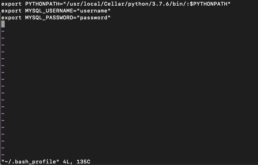
Let's update our bash profile with a faux username and password for a MySQL database using the VIM skills we have learned.
$ vim ~/.bash_profile
This is now what our .bash_profile looks like, assuming it was blank previously.
Let’s now source our .bash_profile to make the changes effective. (It's easy to forget this step!)
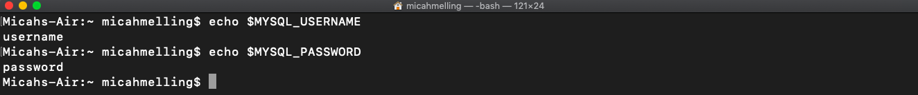
$ source ~/.bash_profile
When we reference MYSQL_USERNAME and MYSQL_PASSWORD, we see the values we assigned in the bash_profile.
We can directly access these variables in Python via the built-in os module. We fire up a Python session, import the os module, reference MYSQL_USERNAME, and exit Python. When we reference MYSQL_USERNAME, “username” is printed in our console. We have successfully referenced a variable in Python set in our bash_profile!
$ python3
>>> import os
>>> os.environ['MYSQL_USERNAME']
>>> exit()
Python Virtual Environments
We have set up our global installation of Python. However, oftentimes we will want to operate in a virtual environment. A virtual environment is a tool to manage an isolated Python instance. The venv function creates a directory that contains the Python executable files along with a copy of pip. Here is an example to illustrate this concept.
Create a directory and make it the current working directory.
$ mkdir venv_sample && cd "$_"
Create a virtual environment called venv-sample.
$ python3 -m venv venv-sample
Let’s now activate our virtual environment. By doing so, any command we issue via the command line will be from our virtual environment.
$ source venv-sample/bin/activate
Let’s try to import the requests library, which we previously installed.
$ python3
>>> import requests
>>> exit()
The foregoing commands produce the following error: “ModuleNotFoundError: No module named 'requests'”. What happened? When we previously installed requests, we installed it in our global Python installation. Since we activated a virtual environment, we are not operating in our global Python installation but a local, isolated one. It’s a vanilla version of Python that only includes the built-in libraries, unless we install more. Let’s now install the requests library in our virtual environment.
$ pip3 install requests
If we now import requests, our code will succeed. However, installing packages one by one is cumbersome, and we would like to complete such a task in one command. We can accomplish this aim with the subsequent command.
$ pip3 install -r requirements.txt
The requirements.txt file houses the names of the packages we want to install along with their version numbers. Naming such a file requirements.txt is standard convention.
$ touch requirements.txt
$ vim requirements.txt
Using vim, let’s add the following lines to our requirements.txt.
pandas==0.25.2
Using the previous command, we can install both of those packages. To note, the package version is optional. If it’s not included, pip will install the most recent version. However, pegging packages to version numbers is best practice.
In our virtual environment, if we had already installed packages without a requirements.txt file, we might still want to create such a file. For example, we might want to build a Docker image that uses an installation of Python that includes these packages (we’ll discuss Docker soon).
To aid in this effort, we can make use of the
$ pip freeze
Pipe the output of pip freeze into a requirements file, verify the file was created, and print it.
$ pip freeze > requirements.txt
$ ls
$ cat requirements.txt
Lastly, when we’re ready to stop interacting with our virtual environment, we can run the following.
$ deactivate
Why would we want to use a virtual environment instead of our global Python version? As we work on more projects and collaborate on shared code bases, we will find our global package versions cannot always fit the needs of individual projects. Projects might rely on differing versions of certain libraries, like numpy and pandas, and simply will not work with new or old versions that might be installed globally. We would have to globally uninstall and re-install libraries at the global level constantly. We might also not remember correct version numbers under such a hectic convention. It can be a mess! We are better served by using virtual environments for each of our projects.
PyCharm Integrated Development Environment (IDE)
As we’ve seen, we can author Python code in a text editor like VIM and run it via the command line. This works well enough, but an integrated development environment (IDE) provides more bells and whistles. For one, a solid IDE will provide linting, which is automatic detection of syntax errors or code not conforming to standards. They also tend to offer code completion. If you have defined a function called main, and you type “m”, you can automatically select that function to autocomplete rather than fully typing it out. Another benefit is that IDEs usually auto-save files, which can be quite useful. Additionally, an IDE typically is easier on the eyes than a plain-Jane text editor.
PyCharm is a powerful IDE designed for Python programming. You can use another IDE if you prefer, but we will be using PyCharm throughout this book.
You can download the free PyCharm community edition: here.
In my home directory, I like to have a directory titled PycharmProjects. (I typically prefer snake_case over CamelCase, but this convention is an old habit for me. Inertia.). In this directory, I keep sub-directories for each of my projects. Let’s create such a structure.
Ensure we are in our home directory; issuing a simple "cd" will accomplish this aim.
$ cd
Create PycharmProjects directory.
$ mkdir PycharmProjects
Create sub-directory as a sample.
$ mkdir sample_project && cd "$_"
Let’s also make a virtual environment called venv, which is a standard naming convention.
$ python3 -m venv venv
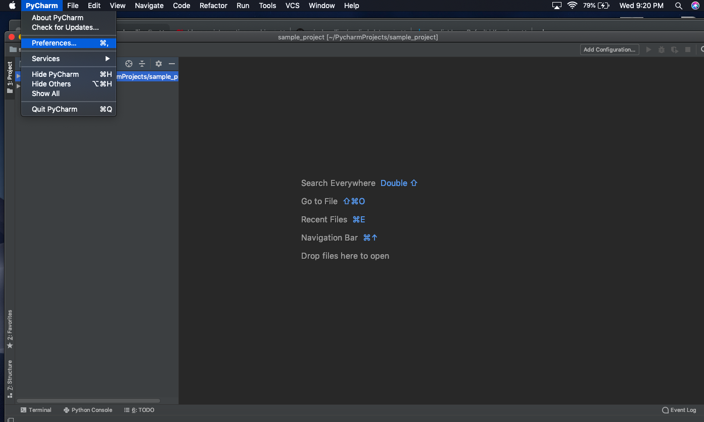
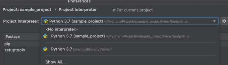
One potential “gotcha” of PyCharm is setting your project interpreter. When we run a script directly from PyCharm, the project interpreter represents the installation of Python that will be used. Let’s see how this is done.
After opening sample_project in PyCharm, click on “PyCharm” in the toolbar and then select Preferences.
Under “Project: sample_project”, click on Project Interpreter. On new versions of PyCharm, the interpreter should default to the virtual environment we just created.
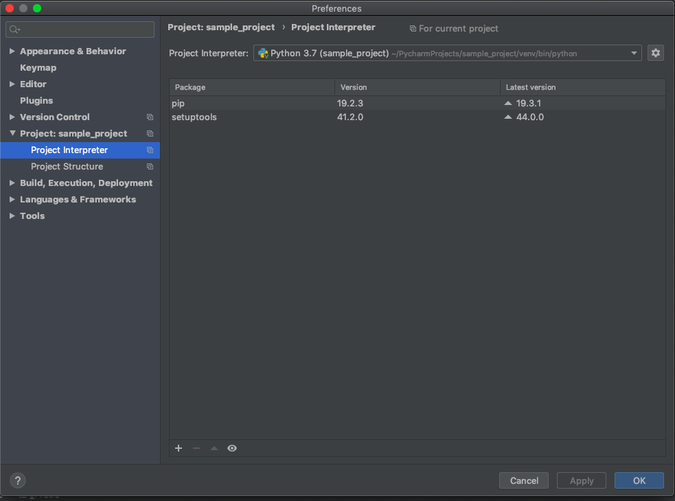
We could also select our global Python installation.
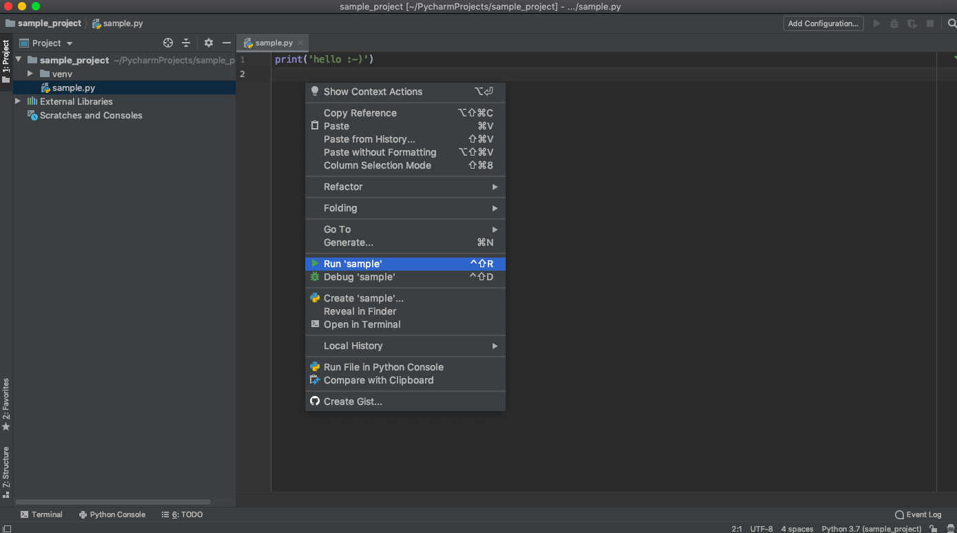
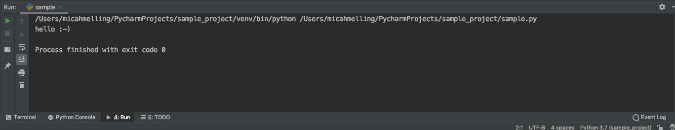
If we create a file called sample.py, insert a simple print statement, right click the opened file in PyCharm, and hit Run, we will execute our script.
After running this file, in the Run section we’ll see the locations of the interpreter and file along with the output.
Though running files from PyCharm can be handy, I generally recommend running scripts, especially production ones, from the command line after you have issued a cd into root. This mimics what you would experience in a Docker container, which we will discuss shortly. If you have a train.py file in a modeling subdirectory and you run that file from PyCharm, "modeling" will become your working directory by default rather than root. This can cause some unexpected behavior in terms of import and file paths if you later run the script from root in a Docker container.
Jupyter Notebooks
While we’re on the topic of Python, I would like to discuss Jupyter Notebooks. We will not use them in this book, and I generally discourage them. Jupyter Notebooks have a number of disadvantages.
- Notebooks files are not conducive to being put in production, either as a REST service of through a job scheduler (they have to be translated).
- Since you can run cells in any order, they lack full reproducibility.
- A proper script should be run end-to-end, not piecemeal (which is common in Notebooks).
- They do not play well with version control (though I know folks are working on a solution).
- Notebooks encourage developers to write code that is not modular.
- Main methods are often not used in Notebooks.
- They encourage you to jam all code into a single file rather than writing local libraries.
- We often see import statements done throughout Notebook cells, rather than all at the top of the file. Such "lazy loading" can be justified in only select cases.
- Notebooks often do not encourage coders to follow PEP8 standards, Python’s standard conventions for authoring code.
- They do not have a debugger.
- Code reviews are important but difficult on procedural, non-repeatable code, which we tend to see in Notebooks.
In sum, Notebooks coddle data scientists and encourage poor software development habits. Do not become reliant on Notebooks. In the long run, you will be better served be writing .py files in PyCharm. This is a piece of advice I wish I would have gotten earlier in my journey as a data scientist.
I have bashed Notebooks. However, they do have a role. When learning a brand new topic, operating in the safety of a Notebook running code line-by-line can be a beneficial pedagogical tool.
Docker
If you want to deploy data science applications, knowing Docker is quite important. Docker essentially allows us to create an isolated environment and package an application with all the necessary dependencies. This enables us to create reproducible environments on which we know an application will run as desired. This ability is vital for both collaboration and for deploying applications in the cloud. Earlier, we introduced Python virtual environments. Think of Docker as a virtual environment on steroids, allowing us to specify dependencies beyond just Python packages. These dependencies are bundled with our code to create a cohesive environment for our application.
If the concept is a built nebulous, don't worry. An example will (hopefully) make Docker's working more concrete.
First, install Docker here. Once Docker is installed, you’ll need to make sure it is running, which can be accomplished on a Mac by simply double-clicking the program in Applications. You should see the whale icon in the top right of your screen. If you click on the whale (a weird statement), it will confirm if the program is running or not.
You can also verify Docker is installed with the following command.
$ docker –version
Docker operates on images. A Docker image is basically a set of instructions for building an application environment. It is often built via a Dockerfile, which is simply another set of instructions in an extensionless file.
Let’s set up the environment we need for our example.
$ cd ~/
$ mkdir docker_example && cd "$_"
Create a simple Python file in our working directory that defines and prints a pandas dataframe. Use whatever text editor your heart desires - my heart desired VIM. Call the file sample.py.
Author a simple requirements,txt file with the following content.
Author a Dockerfile.
Let’s walk through each line of the Dockerfile.
We start from a base Python image provided by Docker Hub. This provides a Linux OS and a Python installation.
The maintainer is a convention that states who authored the Dockerfile.
Make a directory called app.
Make app our working directory.
Move everything in the current working directory into the app directory. In this instance, we are copying sample.py
and requirements.txt into the app directory.
Use pip to install the packages in our requirements file. We disable the cache used by pip to make our image smaller.
The ENTRYPOINT sets the image’s default command. In our case, our image will automatically fire up a Python interpreter.
There's a couple of lines we should add to a production Docker image (e.g. not running our entrypoint as a root user), and we will add those in a later chapter.
Let’s now build our Docker image! The -t flag allows us to tag our image with a name; in this case, we call it "test". To note, the build command will automatically pick up our Dockerfile since it is in our current working directory.
$ docker build -t test .
If we check what Docker images we have, we’ll see we have the test image we recently created and the base Python image we used in our Dockerfile. When we referenced that base image, Docker went out and downloaded it on our machine for us. How nice of Docker.
$ docker images

Now that we have our image, we can use it! The run command fires up a Docker container. A container is an executable package - it's where code can actually be run. Basically, a container is a running image. Think of it as an isolated machine.
$ docker run --rm -it test
Running the foregoing command fires up a Python interpreter for us. Let’s write the following lines of code.
>>> # import pandas, which was in our requirements file
>>> import pandas as pd
>>> # importing requests will result in a ModuleNotFoundError since it was not in our requirements file
>>> import requests
>>> # import the built-in os module
>>> import os
>>> # we can confirm the current working directory is /app, as specified in the Dockerfile.
>>> os.getcwd()
>>> exit()
We can also directly run sample.py in Docker. The command will print our dataframe, as declared in the script.
$ docker run --rm test sample.py
Alternatively, we could override our entrypoint and fire up a bash terminal to execute commands within our container.
$ docker run --rm -it --entrypoint /bin/bash test
$ ls
$ python sample.py
We confirm that our Docker container is basically just an isolated compute environment, with the details defined by our Dockerfile. We're able to run an ls and see our files. We also can fire up our Python interpreter and run code.
In our Docker run command, you might have noticed we have the flags --rm and -it. The --rm flag tells Docker to remove the container when the application finishes. The -it flag makes the session interactive and takes you straight into the container. To make this more concrete, let’s run Docker run without those flags. First, we shall check what containers we have.
$ docker ps -a
Assuming you had no existing containers, this command will show no containers.
Run docker run without the previous flags and check with containers we have.
$ docker run test
$ docker ps -a
You’ll notice two items. First, we were not taken to a Python prompt since we did not have the -it flag. (The -it flag doesn't really do anything for a command like "docker run --rm test sample.py" since we are just running a script directly and not doing anything interactively). Second, we have a container remaining on our machine.
We shall remove the container manually. To note, your Container ID will likely be different from mine. This ID is found after running
$ docker ps -a
$ docker rm ea3fe1653146
Likewise, if we wanted to remove our Docker images, we could find the Image ID and run a "rm" on it. To note, your image ID will likely be different from mine.
$ docker images
$ docker rm 4ab7f9a9706f
Amazon Web Services (AWS)
Amazon Web Services (AWS) is the current leader in cloud computing. AWS provides a number of incredibly useful tools for full stack data science, including hosting databases and deploying APIs. We will cover multiple services throughout this book. For now, we focus on getting set up in AWS.
Important note: While some of the services we will use will be free-tier eligible in AWS, some are not. By going through all of the examples in this book, you are likely to incur charges. Those cases will be called out in the book. To mitigate charges to only a few dollars total, you can terminate the instances after you work through the provided examples.
Start by creating your AWS accounthere. You will also likely want to add a credit card to the billing section as not everything we do will be free-tier eligible. Likewise, I recommend turning on multi-factor authentication for an added layer of security.
At this stage, you have created your root account. Beware! It is incredibly powerful. We actually almost never perform actions with our root account since it is so potent. Rather, we create users with certain permissions. We can accomplish this task with the Identity and Access Management (IAM) service in AWS. For our purposes, we will create two users. The first is an administrator account. This is a powerful account, though less powerful than the root account. We will also create an even less powerful account with only access to the services we need for our specific use cases within our application.
To learn how to create your non-root users, watch the following videos.
As stated in the previous video, we assigned some pretty broad permissions to our churn_model user. This is necessary because we will use this account to work through some tutorials in future sections and chapters. This really is a "book project" account rather than a pure "data science project" account. Generally, we want accounts to only have access to project-specific resources in AWS, not full services. Later in the book, we will use Pulumi to manage our infrastructure as code (i.e. literally writing code to create and permission AWS resources ). As an example, the following script can be used after setting up Pulumi to initiate project resources and a project user. We'll cover this topics more in Chapter 14.
Pulumi has a limitation in this script: we can't get the actual strings of the key and secret to automatically upload them. We can export those items, retrieve them via the command line, and then manually update the secret. Using the exported names in the script above, we can accomplish that with the following commands:
$ pulumi stack output secret_key --show-secrets

        $ pulumi stack output access_key
AWS Security Stance
Cloud security is important. For obvious reasons, we don't want our environment to be hacked or exposed. We can adopt the following security protocols to give us a strong security posture.
- Practically never use the root account. Reasons are discussed previously.
- Use a specific admin account for performing administrative tasks.
- Enforce multi-factor authentication when users sign into the AWS console.
- Require users to create strong passwords. This can be enforced in the account settings of the IAM service.
- Store credentials in a password manager, not in emails or text files. We will use AWS Secrets Manager for this purpose.
- Create focused permissions for users (i.e. grant least-privileged access). Permission sets should generally be managed by an IAM group. For example, all data scientists belong to the data science group and, therefore, have the same permissions. Better yet, we might have a group per project. Data scientists will have to manage multiple API access keys in such a scenario, but this very well could be a fine tradeoff for improved security. The latter is the paradigm we will employ in this tutorial.
- As much as possible, limit programmatic access from access keys. These keys are powerful. When access keys are in use, be sure to rotate them frequently.
- Separate console and programmatic access if at all possible. For instance, each data scientist will have evergreen access to a single account with console-only access. This account will have permissions to two AWS services: CodeCommit and Secrets Manager (well, technically specific secrets in Secrets Manager). CodeCommit is for git repos. Secrets Manager is a secure password manager. Our sample project involves developing an application to predict the probability of customers churning. This project contains AWS services a data scientist might need (e.g. S3 buckets, additional Secrets Manager secrets, etc). The data scientist can gain programmatic access to these resources by logging into AWS, going to Secrets Manager to access the secrets to which they have permissions, finding the appropriate project-specific keys, and placing them in a temporary terminal environment (not in a bash profile). Therefore, at any given time, the API access keys on a local machine only have access to a small set of resources and only persist as long as the terminal session is alive (tell data scientists to kill the terminal session when work is done). This is more secure. If they want to work on a different project, they switch out the keys to those of the appropriate project. Likewise, if a data scientist needs console access to project resources, we could create a separate console-only account. The console account will be protected with the discussed password requirements and MFA protocols. This account might have slightly broader permissions as we don't need to or want to make API calls for all services. Sometimes, we just want to view what has happened or is happening (e.g. the execution of a CI/CD pipeline via CodePipeline). Overall, this separation makes individual accounts less powerful and allows us to fine-tune permissions.
- Use an in-house, private Python library to standardize interactions with AWS. This will enforce certain protocols when working with AWS, helping to ensure compliance and security standards. In the previous step, we architected a system where a data scientist has a single set of AWS access keys in their local environment at any given time. The library, in this case, is an installable Python package (i.e. we can use pip to install it), which will look for those keys when creating the AWS client to make API calls.
- Run workflows in AWS using execution roles, which are securely granted temporary credentials at run time.
- Grant execution roles least-privileged access.
- Ensure that security groups have proper inbound rules.
- Generally, create new a security group per cloud resource/
- Turn on CloudTrail for auditing.
- Create a separation for development, staging, and production environments.
An Aside on Security
A tradeoff exists between security and efficiency. If we lock away our data in a server and throw away the SSH key, we have perfect security since no one can access the data. However, we have zero efficiency. Conditional on your specific use case, you need to find the right balance between security and efficiency. This will be influenced by the nature of your data, the scope of your application, and the level of required collaboration (i.e. the more people involved, the more risk involved).
AWS CLI
If we want to interact with AWS via the command line, we need to install the AWS CLI. We can do this with Homebrew.
$ brew install awscli
Verify the installation.
$ aws --version
Configure the AWS CLI by following the command prompts. To note, your default region can be easily found in the querystring of the URL for your management console. Further, we downloaded the appropriate keys in the second video in a previous section. You can regenerate and download a new set using your administrator account i f needed. Be sure to use the keys for the churn_model user.
$ aws configure
Let’s now use the CLI to interact with S3, the Simple Storage Service. S3 allows us to store files of any kind. We shall create a bucket. Think of it like you would a directory on your local machine where you organize files.
Make a bucket, which must have a globally unique name.
$ aws s3 mb s3://micah-melling-sample-bucket
Verify the bucket has been created.
$ aws s3 ls
Create a sample file, place it in our bucket, and verify it was uploaded.
$ touch sample.txt
$ aws s3 cp sample.txt s3://micah-melling-sample-bucket/
$ aws s3 ls s3://micah-melling-sample-bucket
Finally, delete our bucket and verify the operation.
$ aws s3 rb s3://micah-melling-sample-bucket –force
$ aws s3 ls
boto3 - The AWS SDK for Python
boto3 is the Python SDK (software development kit). it's just a library that you can pip install.
$ pip3 install boto3
boto3 allows you to programmatically interact with AWS services from Python. We won't cover boto3 now - you'll have to hold your excitement until a future chapter. For boto3 to work properly, you need to have AWS_ACCESS_KEY_ID and AWS_SECRET_ACCESS_KEY as environment variables in your bash profile. These are the same keys you used to configure the AWS CLI. For help doing this, review the section in this chapter called "The Power of the Bash Profile".
MySQL Workbench
MySQL Workbench is a graphical user interface client for MySQL, the database we will be using in this book. It provides a deep set of tools to help manage your database and to run adhoc queries. We will use this tool in later chapters once we have our database set up. You can download it here.
Postman
Postman is an API development environment. We will use it to interact with the machine learning API we will develop in later chapters. You can easily download the tool here.