Chapter Introduction: Model Calibration
Model calibration is a crucial yet often overlooked topic in machine learning. Calibrating the probabilities of classification models means they can be interpreted as direct confidence levels. For example, if we predict a person has a 40% chance of churning, we want that to actually mean 40%. This might sound confusing: when would a model say 40% probability but not mean it? The reason is that some models have idiosyncrasies in how they produce probabilities. For instance, random forest models tend to push probabilities toward the middle of the distribution and are less likely to predict probabilities at the extremes (e.g. 5% or 95%). The cardinality of the predictions is still valid, but the out-of-the-box calibration could likely be improved. Of note, one of the benefits of logistic regression is the probabilities are naturally pretty well calibrated.
Producing calibrated probabilities is oftentimes extremely important. In most cases, I would submit that we care much more about the predicted probability than just the plain predicted class. For instance, if Person A has a 2% probability of churning and Person B has a 47% probability of churning, we likely don't want to treat them the exact same, even though they are both predicted to not churn. If we have properly calibrated the probabilities, we can create interesting subsets of our predictions that map to actions. Here is an off-the-cuff example for our churn project:
- 0-10% probability: no action
- 10-40% probability: email message
- 40-60% probability: text message
- 60-95% probability: phone call
- 95-100% probability: no action - considered a lost cause
In the following sections, we will delve into ways to properly calibrate probabilities. This topic is often new to many data scientists, but the methodologies are pretty straightforward.
Calibration Plots
A simple way we can assess model calibration is via a calibration plot. The following code will produce the subsequent calibration plots. You'll also notice we write out the raw data that comprises the visual.
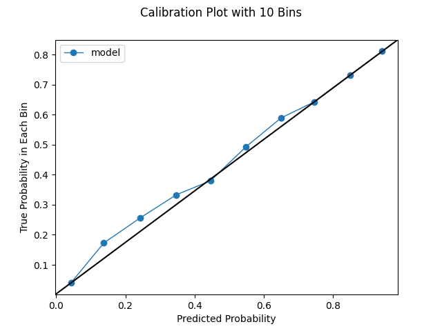
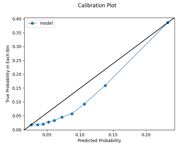
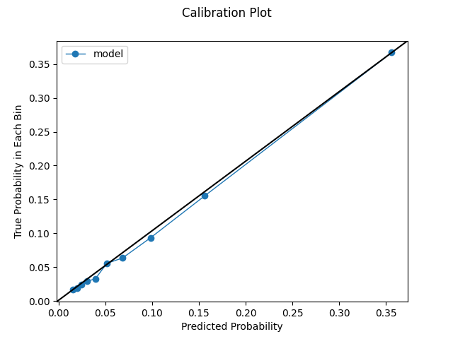
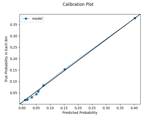
The below calibration plot segments our probabilities into 10 bins, using the results from an uncalibrated Extra Trees model constructed on our churn data. To note, we may not always be able to get the requested number of bins based on our prediction distribution. The dashed line represents a classifier that would score perfectly based on this plot. The plot essentially answers a question such as the following: when we predict, say, 10% probability, does churn happen in 10% of cases based on the real data? For this type of evaluation to occur, we need to aggregate our data to some degree, hence the binning. Behind the scenes, the code is sorting predicted probabilities from highest to lowest, cutting them into the desired number of bins, and calculating the real churn rate within each bin. In sum, we observe that our model has pretty decent calibration out of the box, though improvements could certainly be made, especially on the higher end of the distribution.
An important note: these calibration plots can be deceptive. By aggregating data, they remove variation. It's actually possible to have a comparatively worse model that has a better-looking calibration plot. These plots can obscure the nuances in the distribution - they are, of course, abstractions. Certain improvements or deteriorations may not be reflected. Likewise, certain distributions may be ripe to just look good in this type of plot. The calibration plots are incredibly useful, but they are not a silver bullet. They must be analyzed in the context of other metrics.
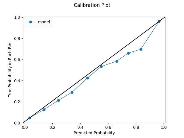
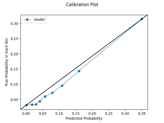
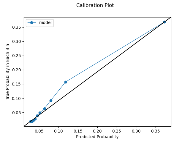
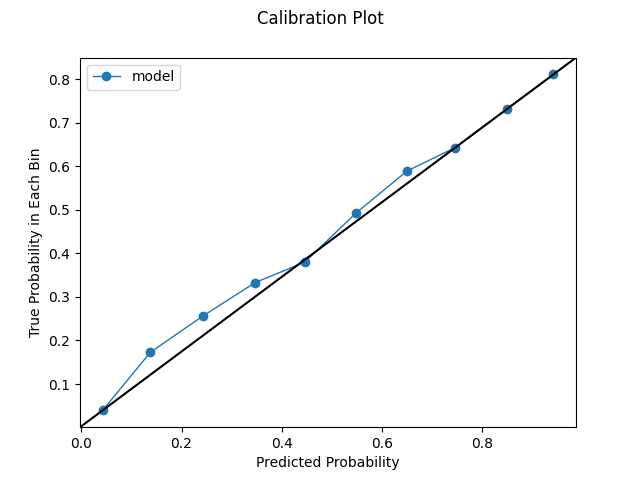
We can also produce a quantile calibration plot. The previous calibration plot ensures we have equal spacing across bins (e.g. 0-10%, 10-20%, etc). With a quantile plot, the bins have the same number of samples, and the range depends on the predicted probabilities. With this view, even a well-calibrated model will not necessarily have a stair-step look. We might see globs of predictions or certain jumps in the distributions. Given the behavior in our data, this may be realistic and even desirable. We care about the points being on the identity line and having proper cardinality. Further, we learn a few items from this view. 1) The model certainly could use some help with calibration. 2) We make a large number of predictions on the low end of the distribution. 3) Conversely, we do not make many predictions on the upper end of the distribution. In fact, we don't make enough predictions above ~0.35 for that part of the distribution to even be reflected on the chart.
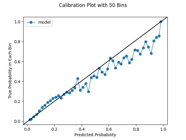
Extension: How Many Bins to Choose
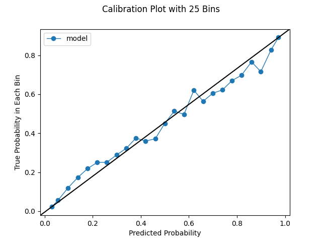
How many bins should we choose for our calibration plots? The default in scikit-learn is 5, which is pretty small. We used 10 in the last section. However, we can increase the bin size, though we could be constrained by our prediction distribution. If we have no predictions in a certain range, we obvious won't be able to produce bins within that range. If we have globs of predictions, or a very conservative model, we may not be able to squeeze out that many uniformly-spaced bins. As we increase the bin size as we're able, we'll see more variation. This is instructive; we've established that a lower bin size can make the performance look deceptively good. However, one of the challenges of increasing the bin size is the charts become a bit more difficult to interpret. We have to look more intently to see what's really happening. With a small number of bins, say 10, we can take a quick look and tell a good model from a bad model. Likewise, with more bins, we will be looking at more noise. Random variation is to be expected, and we shouldn't necessarily take this to be a bad thing. It's simply an artifact of working with real data and making predictions. In general, we should look at different bin sizes. The below series of charts shows the impact of increasing the bin size.
CalibratedClassifierCV
The most effective way to calibrate our models is by using scikit-learn's CalibratedClassifierCV. We can simply wrap our model inside the CalibratedClassifierCV using the base estimator_argument. Using the CalibratedClassifierCV can help our model predict probabilities that can be interpreted as direct confidence levels. In fact, we showed how to configure the CalibratedClassifierCV in chapter 10. There are two general ways we should implement the CalibratedClassiferCV; each ensures we calibrate on different data than we train on.
- We create a validation set from either our training data or our testing data. In such an instance, we would have training, validation, and testing datasets. We would train on our training set, calibrate on our validation set, and test on our testing set. We want our calibration to be disjoint from our training, and we always want to leave our test set only for evaluating our model. If we take this approach, we need to pass "prefit" into the cv argument to tell the classifier that the base_estimator has already been fit.
- We perform the calibration during our normal cross validation. We place a raw, untrained model callable in the base_estimator argument within the CalibratedClassifierCV, and scikit-learn allows us to tune the parameters in this nested space. Some of the parameter grids in chapter 10 reflect this method. One of the benefits of this approach is that our calibrator models will be trained on more data.
Which of the previous options should we choose? In our implementation in chapter 10, we chose to do the calibration during cross validation. Using this strategy, we are finding the best calibrated classifier, per our scoring metric and judged by cross validation scores. By performing post-hoc calibration on a validation set, we are doing something subtly different. During cross validation, we are finding the best model per our scoring metric and then we are calibrating it. The cross validation approach is more direct: we are optimizing for the hyperparameters the result in the best calibrated classifier. This methodology actually makes a lot of sense. If we want to use a CalibratedClassifierCV as our final estimator, we should ideally optimize our hyperparameters with this in mind. However, this approach comes with a cost: greatly increased computational complexity. This drawback will make more sense once we explain exactly how the CalibratedClassifierCV works.
Let's say we are using five-fold cross validation during our hyperparameter optimization routine. Let's also say we leave the defaults of ensemble=True and cv=5 in the CalibratedClassifierCV. With these settings, we will actually fit 50 models per hyperparameter configuration! Without the CalibratedClassifierCV, we would only fit 5 models per hyperparameter configuration. Without question, the use of calibration within cross validation greatly increases our run time. Why exactly? By setting ensemble=True and cv=5, we are fitting an ensemble of five model pairs that all have their predictions averaged. This ensembling improves our calibration. Below is an example of how this would play out for one cross validation split. In our example, the below process will be done four more times since we have specified five-fold cross validation for our hyperparameter optimization routine.
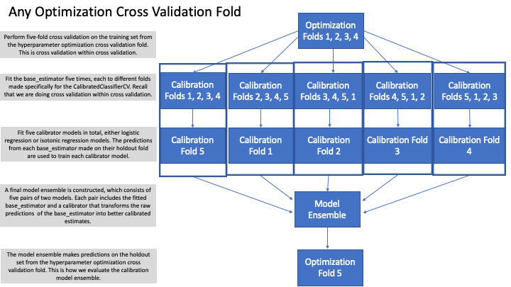
While this may seem like overkill at first blush, the process makes sense and is necessary. The outer loop of cross validation is necessary to try different hyperparameter configurations in our base_estimator, to get multiple test set evaluations, and to obtain an average score on the holdout data. The inner loop of cross validation is required to train the calibrator ensembles since we should not use the same data for training as we do for calibration. Finally, the outer loop and the inner loop must interact, as we need the outer loop's holdout data to evaluate the calibrator model ensemble constructed in the inner loop.
That said, turning off the ensemble is possible. In such a case, we only have one pair of models (i.e. base_estimator and associated calibrator) rather than an ensemble of 5. This will decrease the training time and the size of the model, though it will likely cost us some predictive power. The nested cross validation is still used to generate holdout predictions that can be calibrated, but only a single calibrator model is then trained.
While using the CalibratedClassifierCV during cross validation makes conceptual sense, we have to grapple with the added computational time. Depending on our compute resources, this might be a major drawback. If we have the available horsepower or a small enough dataset, the cross validation approach could be a wise choice. However, when we have limited compute power and / or very large datasets, going with post hoc calibration on a validation set approach could be a smarter use of resources.
A potential downside of using CalibratedClassifierCV is that the base_estimator is never actually fit on the entire training set due to the ensembling. In every ensemble model, a portion of the data is left out. This might be a dowside (hence the "potential" qualification) or it might also serve as useful tenacity against overfitting.
As alluded, there are two types of calibration we can use: sigmoid and isotonic. For both cases, a new dataset is created, and a new model is fit for calibration purposes. The single feature in the calibrator model is simply the base_estimator's predictions, and the target remains the original target. We are basically re-predicting the target using the output of our base_estimator, allowing the calibration to re-weight and correct the calibration of initial predictions.
- The sigmoid method is also referred to as Platt Scaling. In this case, we use a logistic regression as our calibrator model.
- The isotonic method uses an isotonic regression as the calibrator model, which fits a piecewise, non-decreasing function. This has the effect of essentially binning our predictions and then interpolating between these bins. To note, this methodology can perform poorly on small datasets.
One of the notable differences between the sigmoid and isotonic methods is the prediction spaces they produce. The isotonic method constricts the prediction space via the binning and interpolation mentioned above. In the case study later in this chapter, when using the cross validation methodology on a test set of 53,657 observations, the sigmoid model produced 53,591 unique prediction values while the isotonic model produced 22,529 unique prediction values. If we use the post hoc validation set approach, we will use less data, which will constrict our prediction space even further as fewer bins can be found. On the test set, the isotonic model produced only 304 unique prediction values in that instance.
One last note: It is possible that using the CalibratedClassifierCV actually hurts our calibration. As we've discussed, the calibration method uses a statistical model. Like with any model, no guarantee exists this model is any good. If we use this post-hoc methodology, we can pretty easily tell if the CalibratedClassifierCV helps or hurts our calibration. We clearly cannot as directly determine this when using the cross validation methodology. If we use the cross validation methodology and our calibration looks off, that would be a clue to train the model without the CalibratedClassifierCV wrapper and then compare the results.
Post-Hoc Calibration on a Validation Set
We've talked about this topic multiple times, but we shall now show it. If we want to run a post-hoc calibration on our best model, we first need to create a validation set in addition to training and testing sets. We can simply do something like the following:
        x_train, x_test, y_train, y_test = create_train_test_split(x, y)

        x_test, x_validation, y_test, y_validation = create_train_test_split(x_test, y_test)
Likewise, we need a simple function like the following to perform the post-hoc actual calibration.
Calibration and Model Evaluation
Model calibration has an intriguing relationship with model evaluation metrics. To have this discussion, we must jump ahead a bit to the main topic of chapter 12, which formally covers model evaluation.
If we care about calibration, we have to use appropriate evaluation metrics when we are optimizing hyperparameters during cross validation and when we are evaluating our model on the test set. Let's say we care about calibration but use accuracy as our evaluation metric (accuracy is not a great choice for other reasons we will discuss in chapter 12). It's possible to achieve better calibration yet have accuracy unchanged. Largely, a metric like accuracy does not reward calibration. It also cares about class labels (e.g. churn vs. no churn).
Let's say we have one observation in our test set, and it belongs to the positive class. Let's also say we have
two models, one we have calibrated and one we have not. Our models give the following probabilistic
predictions:
- Calibrated Model: 0.45 Uncalibrated Model: 0.20
Given a cutoff of 0.50, both predict the observation to be in the negative class, which is incorrect. However, the calibrated model is less incorrect than the uncalibrated model. The calibrated model gave the observation a noticeable higher chance of being in the positive class. Both models have the same accuracy, but the calibrated model gives a better probabilistic estimate. Accuracy will not reflect this better calibration but instead will say the models perform the same. If we care about calibration, we have to supply an evaluation metric that also cares about calibration. The best two options are log loss and brier score.
Log Loss and Brier Score
Log loss and brier score are scoring metrics that penalize predictions that are confident yet wrong. For both metrics, lower scores are better. The brier score returns a value between 0-1. Log loss does not have a predefined scale; we can only compare values. We cannot assert beforehand that, say, a log loss of 0.20 is "good". We can only compare it to scores from other models.
Given the example in the previous section, the calibrated model would have received a lower log loss and brier score compared to the uncalibrated model. Both were wrong, but the uncalibrated model was more confidently wrong.
Below is an illustrative Python script to fill out this discussion. In this script, we make three sets of predictions, each progressively more incorrect. We compare the log losses and brier scores of the "slightly more wrong" predictions and the "even more wrong" predictions to the first set of predictions. We see that the brier score gives more of a penalty to the "slightly more wrong" predictions. However, log loss provides a much steeper penalty to the "even more wrong" predictions. For probability predictions that are way off, log loss will do the most to slap such errors on the wrist. This is a desirable trait. In general, the brier score is gentler than log loss.
A Case Study Comparison of Calibration Methodologies
We've talked a lot about different calibration strategies. In this section, we test them all on an Extra Trees classifier and see how they compare. To note, the results are highly dependent on this dataset and model. The "best" strategy will change based on these two factors.
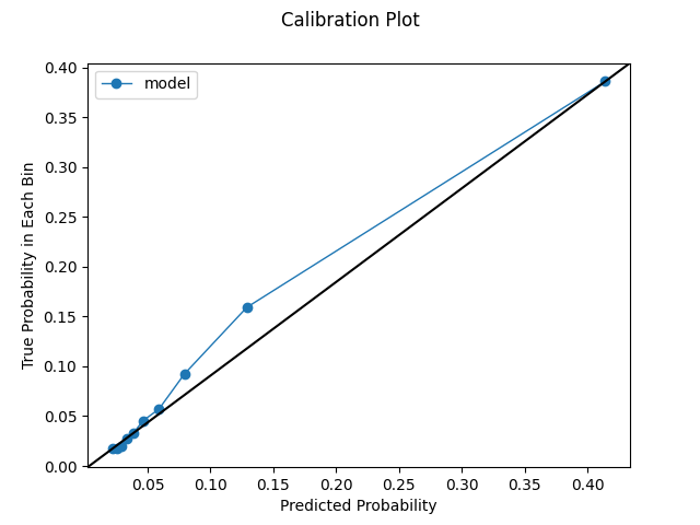
Uncalibrated Model. The uncalibrated model frankly supplies pretty good calibration. The uniformly-spaced calibration plot is pretty solid, and the log loss is competitive with the calibrated models. To note, the uniformly-spaced calibration plot is a bit deceptive compared to subsequent plots. Even though we requested 10 bins, the predictions are distributed in such a way that can only accommodate 6 bins given our spacing rules. This makes the plot appears smoother somewhat arbitrarily. Additionally, the quantile view displays some weaknesses. We make a large number of predictions below 0.10, and many of these could certainly use better calibration. The cardinality is decent, but the calibration could certainly use some work.
log loss on test set: 0.2425
Uniform Calibration Plot
Quantile Calibration Plot
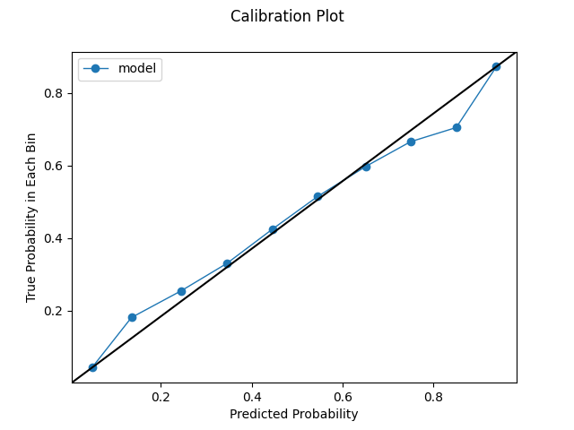
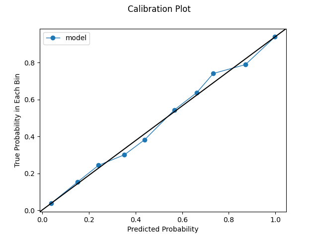
Model calibrated during cross validation using the sigmoid method. We see an improvement through using this mechanism. Our uniformly-spaced calibration plot mostly hugs pretty close to the ideal identity line. We also get a fuller distribution. Notice how we can get our requested 10 bins and how the x-axis has a bigger range. Likewise, we see some improvements in our quantile plot. We still observe a glob of predictions below 0.05, but the calibration shows improvement after this point.
log loss on test set: 0.2379
Uniform Calibration Plot
Quantile Calibration Plot
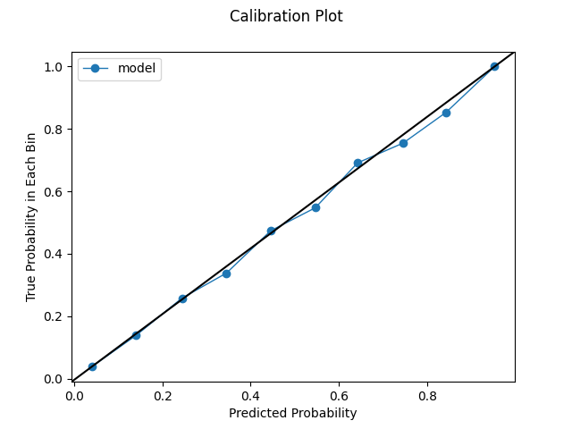
Model calibrated during cross validation using the isotonic method. We get a slight improvement in our log loss with this strategy. The uniformly-spaced calibration plot looks quite good. Again, remember that these plots can be a bit deceptive as they remove variation via aggregation and create a smoothing effect. However, it's still pleasant to have such nice-looking calibration. Likewise, our quantile plot shows some improvements as well.
log loss on test set: 0.2373
Uniform Calibration Plot
Quantile Calibration Plot
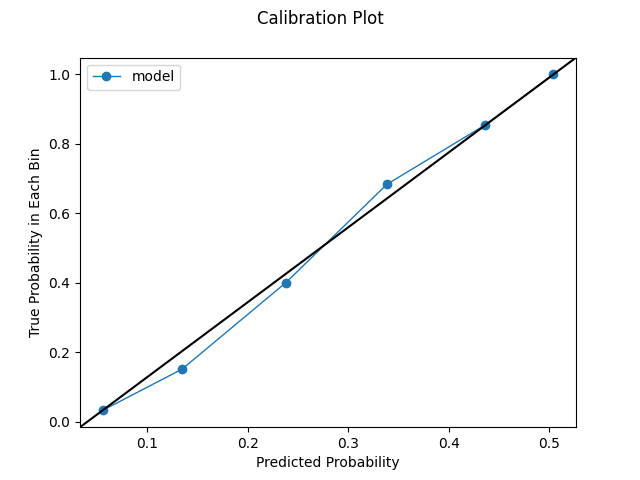
Model calibrated post hoc using the sigmoid method. Employing this technique improves our log loss even more. Our plots actually look a little worse compared to the previous ones. As discussed, this plots are not a panacea. They can be a bit deceptive in some ways. Looking at our plots in conjunction with the log loss metric is key.
log loss on test set: 0.2317
Uniform Calibration Plot
Quantile Calibration Plot
Model calibrated post hoc using the isotonic method. We get a marginal improvement in our log loss. Our plots also look pretty solid.
log loss on test set: 0.2315
Uniform Calibration Plot
Quantile Calibration Plot
In sum, we can see how using different calibration strategies can impact our model's predictions. Again, how this plays out depends on our model and our data.
One-Column Binning
Earlier in the chapter, we binned probabilities based on a uniform or quantile distribution. However, we could find natural breaks, or bins, in our probabilities by using one-column binning. Such results could provide useful insight into our model and help us appropriately map actions to probabilities. To perform this analysis, we need to supply the desired number of bins and use the following code.