Chapter Introduction: Data Wrangling
Data wrangling is the phase where we clean our data and engineer features. During our data exploration step, we identified data quality issues. We need to write functions to correct these issues. Likewise, we might be able to develop new, useful features from our existing data, which can sometimes greatly increase our model's performance. That process is aptly named “feature engineering”. Together, these steps are often referred to as "preprocessing".
A classic cliche is that a data scientist spends 80% of their time on wrangling. In some cases, this is absolutely true. Certain datasets are pretty wicked and require substantial clean up and munging. However, if we write modular and loosely-coupled code, we will be able to repurpose functions across projects. This is a major time saver. We'll always have to author bespoke code, but we should also focus on building a reusable code base over time. We will eventually reap notable time savings.
As established, we primarily author wrangling functions for two purposes: 1) to clean data and to 2) engineer new features. The former is mandatory (well, if we actually care about model quality) and the latter is optional yet important. An important caution: don't initiallyget mired too deeply in feature engineering. Up front, engineering a ton of features can be tempting; however, we initially have no feedback on whether our features will provide any lift. My recommendation is to first only engineer a select few features that we believe could be useful based on subject-matter expertise. Then, run the initial models and inspect feature importance scores. This will provide feedback on our initial feature engineering work. If none of the features are useful, then we should go back to the drawing board. If the features are predictive, that serves as validation of our work and a potential springboard for engineering more features. Work iteratively and incrementally.
In this chapter, we will be inserting code into helpers/model_helpers.py. You'll need to create to this file.
Cleaning Functions
We need to clean up flaws in our data before feeding it into our model. The below are the cleaning functions we will employ.
We don't have too many functions - our cleaning is pretty straightforward. We won't have to write our own cleaning functions in some cases as scikit-learn provides quite a bit of useful preprocessing functionality. For example, we have some features with zero variance, and we can have scikit-learn remove such features.
Engineering Functions
Alright, we have written the functions to clean our data. We shall now author functions to engineer new features.
Transformer Classes
In chapter 10, we will discuss the concept of hyperparameter optimization. At a high level, this process involves tuning the knobs of an algorithm to maximize predictive performance. Oftentimes, hyperparameter optimization is performed to tune the parameters of only the machine learning model. For instance, if we're training a random forest, we would be best served to tune the maximum depth for each decision tree (see discussion of trees in chapter 2 if you need background). However, why wouldn't we want to tune the parameters of our data cleaning and feature engineering? How we clean our data and engineer our features can have an immense impact on model performance. We want to find the version of the cleaning and engineering functions that maximizes predictive performance. More specifically, we want to find the optimal combination of parameters across the preprocessing functions and the machine learning model. Our preprocessing and model parameters can interact and influence each other. We want to tune them in concert. This idea might be a bit foggy. Don't worry - it will be made more concrete in chapter 10.
If we're using a preprocessing function from scikit-learn (more on those later), we can easily tune the relevant parameters (e.g. using SimpleImputer to determine if we should fill numeric nulls with the mean or the median). However, if we have authored our own preprocessing function, we can't natively tune it in a scikit-learn pipeline. To accomplish this aim, we need to convert the function into a class that inherits from a couple of scikit-learn's base classes.
Below are two preprocessing classes with tunable parameters. One allows us to determine if we should or shouldn't take the log of our numeric columns. The second allows us to determine if we would be better served by combining sparse category levels. In the fit section, we create a mapping for each column and its sparse categories. In the transform section, we perform the actual collapsing of category levels by column. This helps to prevent feature leakage - that will be examined more later in this chapter.
To note, I was first introduced to this idea in the excellent book Hands-On Machine Learning with Scikit-Learn and TensorFlow.
Planning for Handling Missing Value
In our dataset, we have missing values. We must address these observations, and we have a few options for doing so.
- Drop the rows with missing data. This is not a great choice unless a row is rampant with missing data.
- If numerical data, impute with a measure of central tendency. This is a simple yet often effective method. One of the advantages is this technique is computationally inexpensive.
- If categorical data, impute a constant value. This approach can be appropriate if we think the missing values represent a distinct category. For example, the category of "missing_value" might be meaningful and tell us something important about the observation.
- If categorical data, impute the most frequent value. This can be a decent bet if we don't think a "missing_value" category is warranted.
- Build a model to predict the missing value. This method can, in some cases, give us a more accurate imputation. However, it could be overkill in some cases, and it's also the most computationally expensive method. We'll have to ascertain if the pros outweigh the cons for using this type of imputation.
At this stage, we won't actually impute any missing values. We want to build this component into our modeling pipeline. This approach has a few crucial benefits. First, it prevents feature leakage. For example, if we want to impute missing numerical data with the mean, we only want to calculate the mean with our training data and not the holdout set of data (called the testing data) used to see how our model will generalize to new data. If we use observations from our testing data, we will be leaking information into our training data, and our model evaluations will be overly optimistic. This means we also cannot split our data into training and testing sets, calculate the means on the training data and then apply those means to missing values on the testing set. Why? During cross validation, part of our training data becomes testing data for a given fold. We'd be leaking information! A second benefit is that we can serialize our modeling pipeline and automatically apply our transformations to new data. For instance, if the mean of Column A is 5, we can save our pipeline so this value is remembered for future imputations. This may sound a bit abstract now, and that's OK. It will all make more sense when we develop our full modeling pipeline in chapter 10.
Planning for Handling Categorical Features
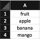
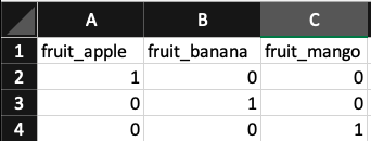
With the models we will build in chapter 10, we cannot feed in features that are encoded as strings. We have to translate them into numbers. The most common way to do this is via one-hot encoding. If a category level is present, the column value is 1. Otherwise, it is 0. An example should make this concrete.
Here is the original column.
Here is the one-hot encoding of the column.
We will implement one-hot encoding via scikit-learn's DictVectorizer class. This has the major benefit of seamlessly handling features our modeling pipeline has never seen before. For example, if the marketing team adds a new source that our model has never seen, the model won't return an error. It will be able to make a prediction without an issue. This is not the case for some like pandas get_dummies. However, to use DictVectorizer, we'll first need to transform our data with the following class (again, we'll do so in our pipeline in chapter 10).
One-hot encoding is fairly intuitive to understand and straightforward to apply. However, it does have one potentially major drawback: we might greatly increase the number of columns in our dataset, and could even end up with more columns than rows. Many modern machine learning algorithms, given proper implementation and tuning, can handle such high-dimensional data well. Even if our algorithm can handle the increase in columns, we will experience a slowdown in the time it takes to train our models since we have added so many columns. An alternative is mean target encoding. This technique replaces the category value (i.e. a string) with the percentage of occurrences in the positive class. This approach may or may not be better than one-hot encoding for any given problem. The only way we can tell is through experimentation.
To make this concept more concrete, we will write a class to implement mean targeting encoding. We have two main points to keep in mind. 1) We need to be sure to not leak any information from our testing set into our training set, including our cross-validation test folds. 2) Related, we will only implement this class in our modeling pipeline (see discussion on null imputation for additional context). To note, this is actually not the implementation we will use in production - we'll identify that in the next section. In this implementation, we are leaking a small amount of information. Can you spot how?
Let's demo this transformer. By looking at the sample data below, in the column called "col", level "a" has a mean of 0.70, level "b" has a mean of 0.5, and level "c" has a mean of 0. We fit our transformer on this dataframe (i.e. perform the calculations) and then transform the dataframe by applying the calculations from the fit step. We see that levels a and b have been replaced with their means! Level c is assigned the overall mean since it falls below our sparsity threshold. We then transform our second dataframe and see the same numbers encoded, even though we don't know the means of a, b, and c in that specific dataframe. We are taking what we know about one dataset and transferring it to a new dataset. This is the exact same concept as training and testing sets for modeling. We only learn on the training set and then apply what we have learned to the test set; we don't learn on the test set. Also, you'll notice there is a new column in the second dataframe. Those values remain unchanged since that column wasn't fitted. (To note, this works the same way as CombineCategoryLevels). Under the hood, this is generally how something like scikit-learn's SimpleImputer works. It finds the mean on the train set and applies it to the test set. This likewise explains how we can persist such learnings (e.g. the mean of a certain column during training) via serialization (using something like joblib). Such values are cemented in the fit step via class attributes so they can be serialized to disk, read back into memory, and applied to new data seamlessly. It's a mechanism for "remembering" values.
Digging Deeper: Planning for Handling Categorical Features
In the previous section, we discussed one-hot encoding and constructed our own class for mean target encoding. However, we have other choices for categorical encoding, found in the category_encoders library. This has a number of options for handling our categorical features. The following are the most applicable encoding methods for our specific situation. All of these implementations can be placed in our modeling pipeline, and select examples will be shown in the next chapter.
- Target Encoder. This works very closely to our target encoder class in the last section. In our implementation, if the category level had below a certain number of observations, the global mean would be used. In the category_encoders implementation, a smoothing parameter is used in conjunction with the category level count. There is no hard cutoff for factoring in the global mean like in our implementation. It will always be a factor, more so for sparse category levels, as long as smoothing is not set to 0.
- Leave One Out Encoder. This works exactly like the Target Encoder but each row's target value is ignored when calculating the imputation for that row. This is the implementation of mean target encoding we want to use!
- M-Estimate Encoder. Again, this is similar to the Target Encoder, but the m parameter sets how much the global mean should matter. When m=0, the global mean has no influence.
- CatBoost Encoder. This method works like the Leave One Out Encoder but with a twist. It assumes that each observation in your training fold is ordered as a time series. Therefore, only previous values are used to calculate the target level's mean. For example, for the 50th example in the training fold, this encoding would only use the first 49 examples in the calculation. This may seem strange, but the goal is to further fight overfitting.
- Generalized Linear Mixed Model Encoder. This is a completely different concept. This method fits a Linear Effects Mixed Model on the target and uses the category levels as the groups in the model.
- Weight of Evidence Encoder. This is another unique approach. For each group, the following calculations are performed. 1) The number of positive cases in each category level is divided by the total number of positive cases. 2) The number of negative cases in each category level is divided by the total number of negative cases. 3) The distribution of positive cases is then divided by the distribution of negative cases. 4) Lastly, the log is taken. The higher the value, the more confident we are the category level skews toward the positive class.
The only way to know if these methods outperform one-hot encoding is through trial and error. The beauties of one-hot encoding are that it is simple to understand, does not risk feature leakage, and often works quite well. The "more advanced" methods methods can risk subtle feature leakage unless we're careful (for example, we should use the Leave One Out Encoder rather than the Target Encoder). Likewise, they might add complexity without much performance lift. Again, these techniques might perform better - we just have to try them out.
A Note on Multicollinearity
If you've taken a stats class and covered linear regression, you're likely familiar with multicollinearity. In fact, you were likely beaten over the head with it. For those uninitiated with the concept, multicollinearity is when multiple features are highly correlated. This can cause issues with the interpretation of linear model coefficients but not necessarily with the predictive accuracy. Likewise, multicollinearity can muddy the interpretation of nonlinear models. When building a model where our main goal is predictive power and not interpretation, we frankly don't care as much about multicollinearity. We want a model to, first and foremost, be able to predict well. We can live with correlated features if we get better predictive power. In Chapter 13, you'll see how we can explain the predictions of our models, even nonlinear ones.